|
|
| Line 231: |
Line 231: |
| We will now expand our example to a system of two coupled ODEs. Still in the same reactor we are now considering the rate constant to be a function of temperature: , with J/(mol) and R = J/mol.K, and is the time-varying tank temperature, measured in Kelvin. Furthermore, the reaction is known to release heat, with J/mol. The time-dependent mass and energy balance for this system is now: | | We will now expand our example to a system of two coupled ODEs. Still in the same reactor we are now considering the rate constant to be a function of temperature: , with J/(mol) and R = J/mol.K, and is the time-varying tank temperature, measured in Kelvin. Furthermore, the reaction is known to release heat, with J/mol. The time-dependent mass and energy balance for this system is now: |
|
| |
|
| | | \[ \begin{align*}\frac{dC_{\sf A}(t)}{dt} &= \frac{F(t)}{V} \bigg( C_{{\sf A},\text{in}} - C_{\sf A} \bigg) - 0.24 e^{-\frac{E_a}{T}} C_{\sf A}^2 \ \frac{dT(t)}{dt} &= \frac{F(t)C_p(T)}{V}\bigg(C_{{\sf A},\text{in}}T_\text{in} - C_{\sf A}(t)T(t) \bigg) - 0.24 e^{-\frac{E_a}{T}} C_{\sf A}^2 (\Delta H_r)\end{align*}\] |
|
| |
|
| where mol/L, we will initially assume constant volume of L and constant inlet flow of L/min. Also, J/(mol.K), the molar heat capacity of the liquid phase system, a weak function of the system temperature. We need an additional initial condition for the temperature differential equation: | | where mol/L, K; we will initially assume constant volume of L and constant inlet flow of L/min. Also, J/(mol.K), the molar heat capacity of the liquid phase system, a weak function of the system temperature. We need an additional initial condition for the temperature differential equation: |
| * mol/L | | * mol/L |
| * | | * |
|
| |
|
| In the code below we will integrate the ODE from minutes up to minutes and plot the time-varying trajectory of concentration in the tank. | | In the code below we will integrate the ODE from minutes up to minutes and plot the time-varying trajectory of concentration in the tank. |
Revision as of 17:24, 18 November 2010
Background
In our course we have learned several ways of integrating a single equation with a given initial condition ; and we have shown that a system of first order ODE's can be integrated: given a set of initial conditions , i.e. is an vector. The course notes covered Euler's method, Heun's method and Runge-Kutta methods.
However, we only coded Euler's method (because it was simple!), but not the others. These other methods have been (reliably) coded in software packages and sophisticated error correction tools built into their algorithms. You should always use these toolbox functions to integrate your differential equation models. In this section we will show how to use MATLAB and Python's built-in functions to integrate:
- a single differential equation
- a system of differential and algebraic equations.
We will only look at initial value problems (IVPs) in this tutorial.
MATLAB
MATLAB's has several ODE solvers available. You can read up more about the implementation details in this technical document.
Python
Like MATLAB, several integrators are available in Python. The integrator I will use in this tutorial is one of the most recent additions to SciPy - the VODE integrator developed at Lawrence Livermore National Laboratories in 1988. It is a good general-purpose solver for both stiff and non-stiff systems.
NOTE: we will use the superior vode Python integrator - it requires a little more code than the other built-in Python integrator, based on lsodea.
Example problem
The example we will work with is a common modelling reaction: a liquid-based stirred tank reactor, with (initially) constant physical properties, a second order chemical reaction where species A is converted to B according to , with reaction rate . One can find the time-dependent mass balance for this system to be:
where mol/L, we will initially assume constant volume of L and constant inlet flow of L/min. The reaction rate constant is 0.24 . We must specify an initial condition for every differential equation: we will let mol/L.
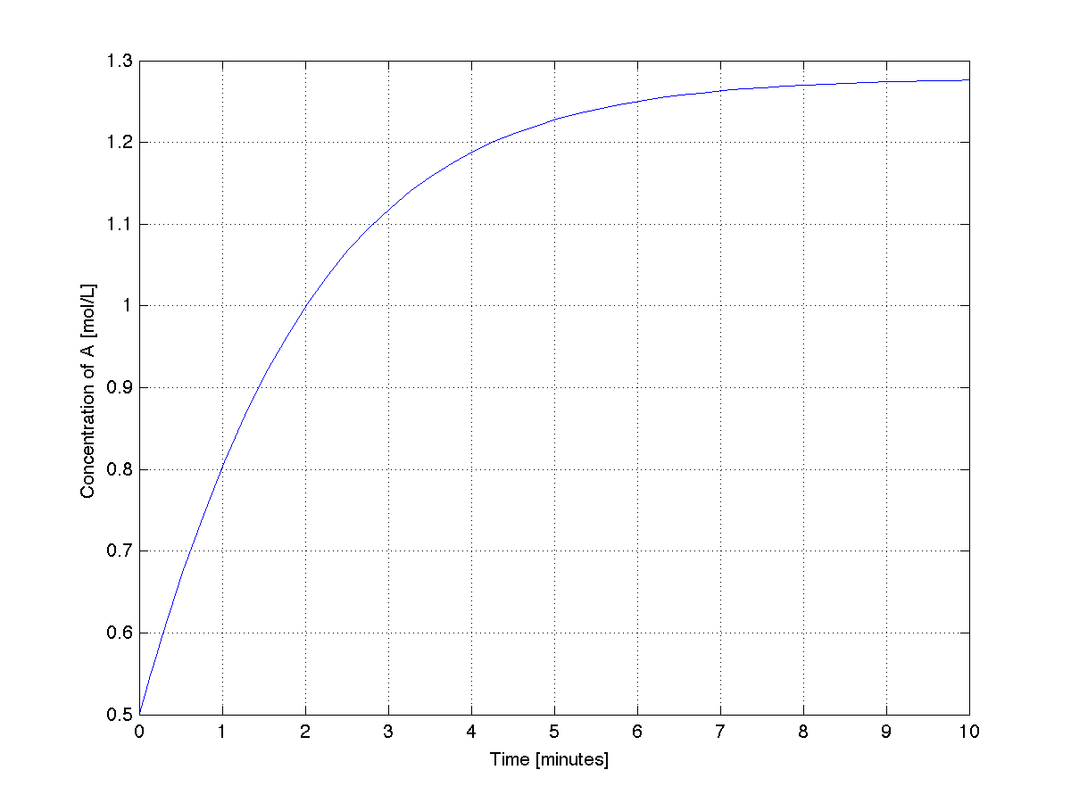
In the code below we will integrate the ODE from minutes up to minutes and plot the time-varying trajectory of concentration in the tank.
| MATLAB
|
Python
|
|
In a file called tank.m:
function dydt = tank(t, y)

% Dynamic balance for a CSTR
%
% C_A = y(1) = the concentration of A in the tank, mol/L
%
% Returns dy/dt = F/V*(C_{A,in} - C_A) - k*C_A^2

F = 20.1;     % L/min
CA_in = 5.5; % mol/L
V = 100;     % L
k = 0.24;     % 1/min

% Assign some variables for convenience of notation
CA = y(1);

n = 1;       % A single, first-order ODE

% The output from the ODE function must be a COLUMN vector, with n rows
dydt = zeros(n,1);
dydt(1) = F/V*(CA_in - CA) - k *CA^2;
In a separate file (any name), for example: ode_driver.m, which will "drive" the ODE solver:
% Integrate the ODE
% -----------------

% Set the time range:
t_start = 0;
t_final = 7.0;

% Set the initial condition(s):
CA_t_zero = 3.2;

% Integrate the ODE(s):
[t, y] = ode45(@tank, [t_start, t_final], [CA_t_zero]);

% Plot the results:
clf;
plot(t, y)
grid('on')
xlabel('Time [minutes]')
ylabel('Concentration of A [mol/L]')
The plot generated from this code shows that the system stabilized after about 6 minutes.

|
import numpy as np
from scipy import integrate
from matplotlib.pylab import *

def tank(t, y):
    """
    Dynamic balance for a CSTR

    C_A = y(1) = the concentration of A in the tank, mol/L

    Returns dy/dt = F/V*(C_{A,in} - C_A) - k*C_A^2
    """

    F = 20.1     # L/min
    CA_in = 5.5  # mol/L
    V = 100      # L
    k = 0.24     # 1/min

    # Assign some variables for convenience of notation
    CA = y[0]

    n = 1        # A single, first-order ODE

    # Output from ODE function must be a COLUMN vector, with n rows
    dydt = np.zeros((n,1))
    dydt[0] = F/V*(CA_in - CA) - k*CA**2
    return dydt

# The ``driver`` that will integrate the ODE(s):
if __name__ == '__main__':

    # Start by specifying the integrator:
    # use ``vode`` with "backward differentiation formula"
    r = integrate.ode(tank).set_integrator('vode', method='bdf')

    # Set the time range
    t_start = 0.0
    t_final = 7.0
    delta_t = 0.1
    # Number of time steps: 1 extra for initial condition
    num_steps = np.floor((t_final - t_start)/delta_t) + 1

    # Set initial condition(s): for integrating variable and time!
    CA_t_zero = 3.2
    r.set_initial_value([CA_t_zero], t_start)

    # Additional Python step: create vectors to store trajectories
    t = np.zeros((num_steps, 1))
    CA = np.zeros((num_steps, 1))
    t[0] = t_start
    CA[0] = CA_t_zero

    # Integrate the ODE(s) across each delta_t timestep
    k = 1
    while r.successful() and k < num_steps:
        r.integrate(r.t + delta_t)

        # Store the results to plot later
        t[k] = r.t
        CA[k] = r.y[0]
        k += 1

    # All done!  Plot the trajectories:
    plot(t, CA)
    grid('on')
    xlabel('Time [minutes]')
    ylabel('Concentration [mol/L]')

|
The reason for the longer Python code is because we have to constructe the vectors that store the time variable and the corresponding concentration output (as a function of that time variable). The MATLAB code builds this vector for us. MATLAB's vectors are very well suited to plotting, but there is a feature that may not be 100% useful:
| MATLAB
|
Python
|
|
Let's take a look at the MATLAB output:
>> t(1:10)
ans =
         0
    0.0805
    0.1610
    0.2414
    0.3219
    0.4780
    0.6341
    0.7902
    0.9463
    1.1213

>> y(1:10)
ans =
    3.2000
    3.0498
    2.9184
    2.8030
    2.7011
    2.5346
    2.4014
    2.2943
    2.2067
    2.1264
MATLAB places the points at unequal step sizes of time. This is what their documentation has to say:
- The MATLAB ODE solvers utilize these methods by taking a step, estimating the error at this step, checking to see if the value is greater than or less than the tolerance, and altering the step size accordingly. These integration methods do not lend themselves to a fixed step size. Using an algorithm that uses a fixed step size is dangerous since you can miss points where your signal frequency is greater than the solver frequency. Using a variable step ensures that a large step size is used for low frequencies and a small step size is used for high frequencies. The ODE solvers within MATLAB are optimized for a variable step, run faster with a variable step size, and clearly the results are more accurate.
|
Let's take a look at the Python output:
>>> t[0:10]
array([[ 0. ],
       [ 0.1],
       [ 0.2],
       [ 0.3],
       [ 0.4],
       [ 0.5],
       [ 0.6],
       [ 0.7],
       [ 0.8],
       [ 0.9]])
>>> CA[0:10]

array([[ 3.2       ],
       [ 3.01656488],
       [ 2.86105764],
       [ 2.72822726],
       [ 2.61403267],
       [ 2.51531912],
       [ 2.42958245],
       [ 2.35480722],
       [ 2.28935862],
       [ 2.23189292]])
The evenly spaced periods of time were by design - see the Python code above. After reading the MATLAB description alongside, you might think the Python integration is inaccurate. This is not true: the Python code we have used here will take multiple steps, of variable size, within each of the delta_t time steps we specified, but the code will only report the values at the boundaries of each delta_t, not the intermediate values.
|
Example with coupled ODEs
We will now expand our example to a system of two coupled ODEs. Still in the same reactor we are now considering the rate constant to be a function of temperature: , with J/(mol) and R = J/mol.K, and is the time-varying tank temperature, measured in Kelvin. Furthermore, the reaction is known to release heat, with J/mol. The time-dependent mass and energy balance for this system is now:
where mol/L, K; we will initially assume constant volume of L and constant inlet flow of L/min. Also, J/(mol.K), the molar heat capacity of the liquid phase system, a weak function of the system temperature. We need an additional initial condition for the temperature differential equation:
In the code below we will integrate the ODE from minutes up to minutes and plot the time-varying trajectory of concentration in the tank.

