Difference between revisions of "Getting started with MATLAB or Python"
| (50 intermediate revisions by 2 users not shown) | |||
| Line 1: | Line 1: | ||
=Introduction to the Command Line= | =Introduction to the Command Line= | ||
*MATLAB IS CASE SENSITIVE!!! For example, '''A''' is not the same thing as '''a'''. This is very important when working with variable and function names. | |||
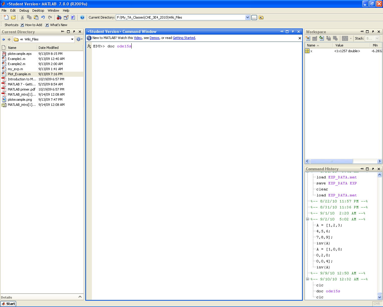
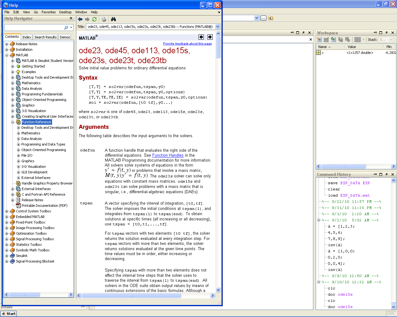
==== | =====doc ''function_name''===== | ||
Brings up information on any built-in MATLAB function (i.e. it accesses the help directory entry). | |||
{| style="border: 1px black;" cellpadding="3" | {| style="border: 1px black;" cellpadding="3" | ||
| Line 133: | Line 11: | ||
!After | !After | ||
|-align="center" | |-align="center" | ||
|[[File:MATLAB_doc_before.PNG|center| | |[[File:MATLAB_doc_before.PNG|center|400px]] | ||
|[[File:MATLAB_doc_after.PNG|center| | |[[File:MATLAB_doc_after.PNG|center|400px]] | ||
|} | |} | ||
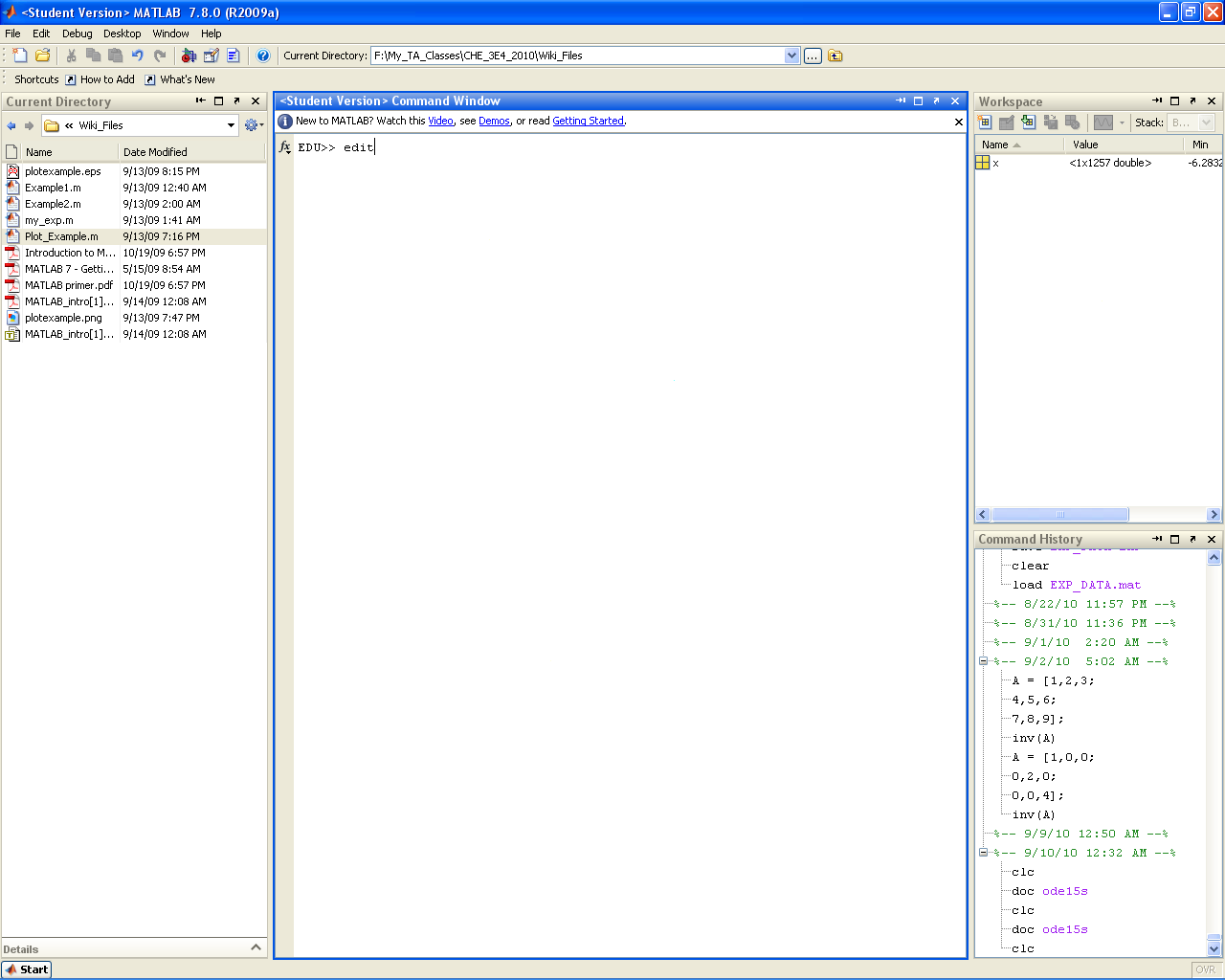
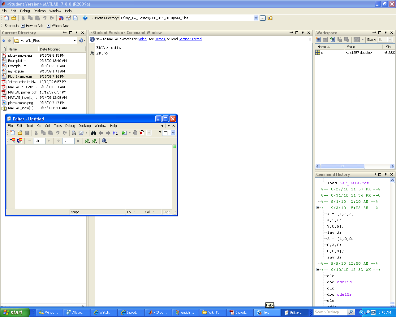
=====edit===== | |||
Opens the text editor | |||
{| style="border: 1px black;" cellpadding="3" | {| style="border: 1px black;" cellpadding="3" | ||
| Line 144: | Line 22: | ||
!After | !After | ||
|-align="center" | |-align="center" | ||
|[[File:MATLAB_edit_before.PNG|center| | |[[File:MATLAB_edit_before.PNG|center|400px]] | ||
|[[File:MATLAB_edit_after.PNG|center| | |[[File:MATLAB_edit_after.PNG|center|400px]] | ||
|} | |} | ||
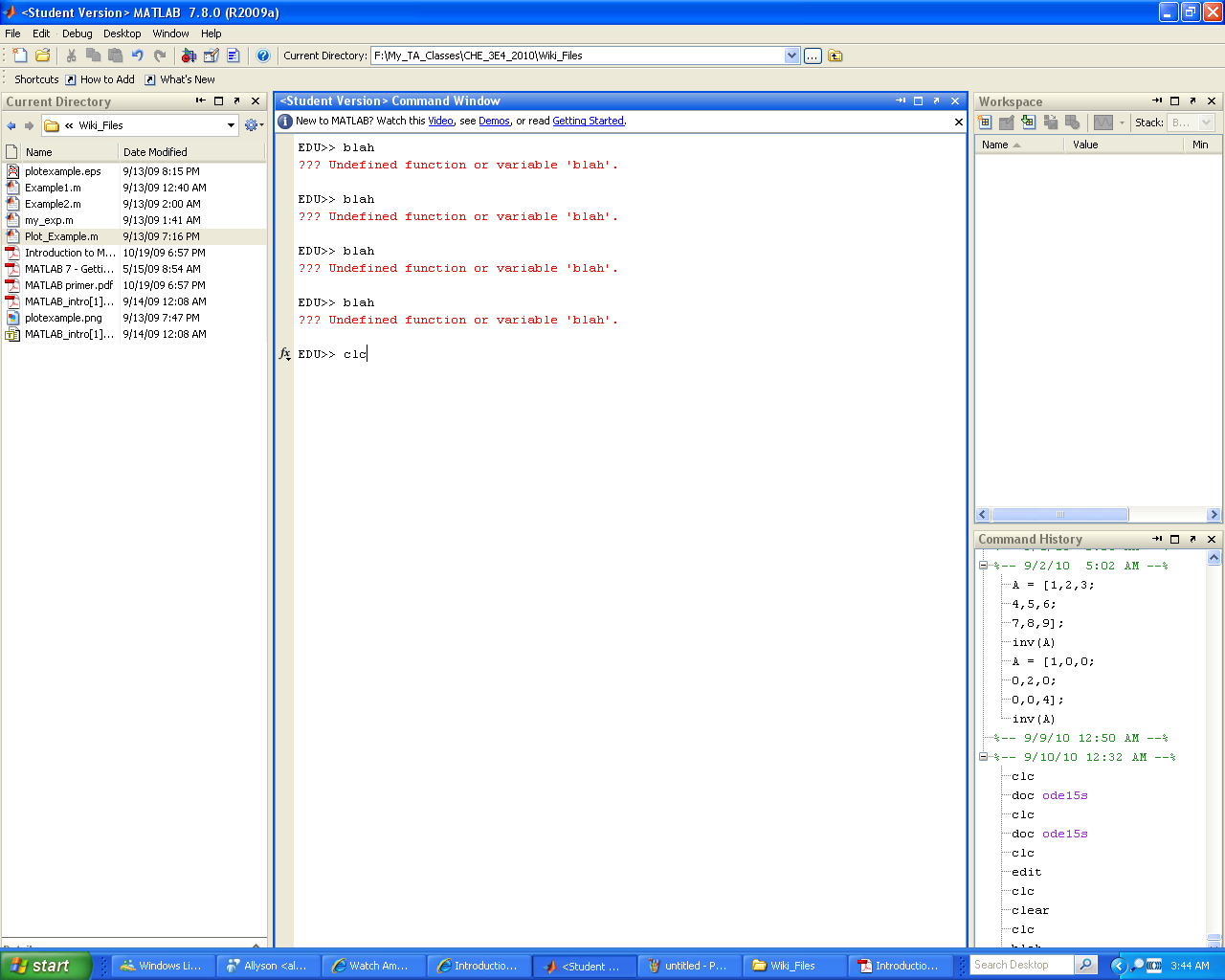
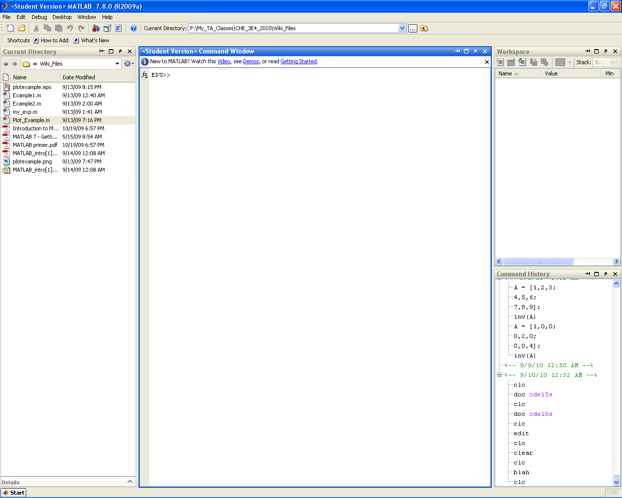
=====clc===== | |||
Clears the screen | |||
{| style="border: 1px black;" cellpadding="3" | {| style="border: 1px black;" cellpadding="3" | ||
| Line 155: | Line 34: | ||
!After | !After | ||
|-align="center" | |-align="center" | ||
|[[File:MATLAB_clc_before.PNG|center| | |[[File:MATLAB_clc_before.PNG|center|400px]] | ||
|[[File:MATLAB_clc_after.PNG|center| | |[[File:MATLAB_clc_after.PNG|center|400px]] | ||
|} | |} | ||
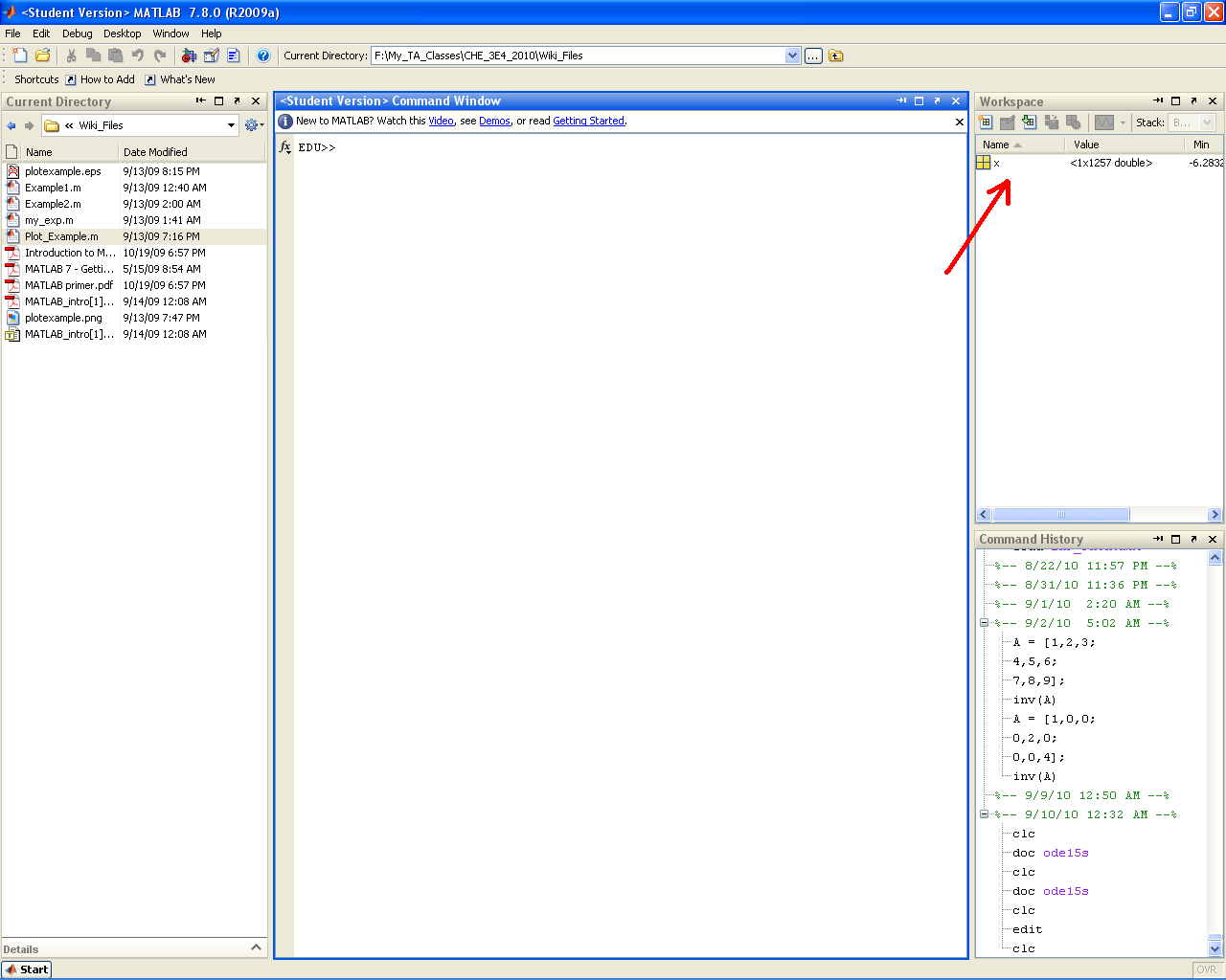
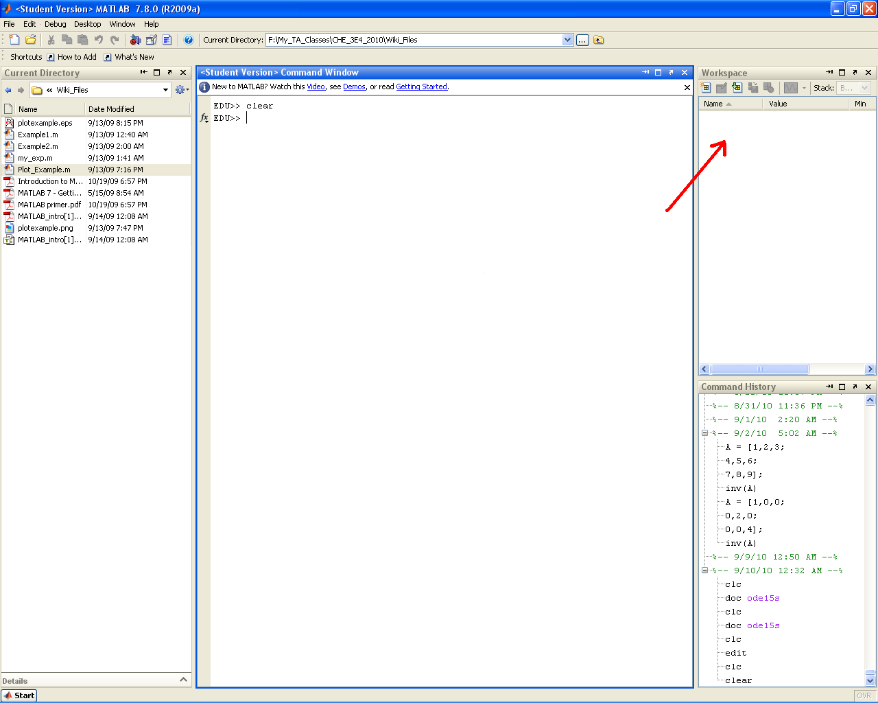
=====clear===== | |||
Clears the variables from the workspace (and from memory) | |||
{| style="border: 1px black;" cellpadding="3" | {| style="border: 1px black;" cellpadding="3" | ||
| Line 166: | Line 46: | ||
!After | !After | ||
|-align="center" | |-align="center" | ||
|[[File:MATLAB_clear_before.PNG|center| | |[[File:MATLAB_clear_before.PNG|center|400px]] | ||
|[[File:MATLAB_clear_after.PNG|center| | |[[File:MATLAB_clear_after.PNG|center|400px]] | ||
|} | |} | ||
=====Built in Functions===== | |||
MATLAB has an array of simple built in functions. Basically all of the rudimentary calculation types that you can think of (sin,cos,exp,etc.) have a built in MATLAB function that may be called at the command line and coded into a script or function file (as the need arises). A few examples are shown in the screenshot below. | |||
[[File:MATLAB_Common_Functions.PNG|center|400px]] | [[File:MATLAB_Common_Functions.PNG|center|400px]] | ||
=====Built in Constants===== | |||
MATLAB also has predefined variables for fundamental constants (ex. pi, Inf, i). Be wary though, as these can be easily overwritten by the user. As a rule of thumb try not to name your variables after any fundamental mathematical constant. | |||
[[File:MATLAB_constants.PNG|center|400px]] | [[File:MATLAB_constants.PNG|center|400px]] | ||
=====fprintf() and disp()===== | |||
fprintf() and disp() provide a means of printing text to the command window. While obviously not useful at the command line (as the example below shows), these statements will become useful when you begin writing your own scripts and functions (either as a means of displaying intermediate results or as a means of tracking down bugs). disp() is a simple display function that prints arrays or strings directly to the command window. fprintf() is a more robust function that allows formatting of the string to be printed as well as output specification (for use in printing to files). The default output is set to the command window. | |||
[[File:MATLAB_fprintf.PNG|center|400px]] | [[File:MATLAB_fprintf.PNG|center|400px]] | ||
=====Semicolon===== | |||
Placing a semicolon at the end of a line of code will suppress any output produced by that line. This (along with fprintf() and break points) can help in debugging code. Unless you are debugging it is good practice to end all lines of code with a semi-colon to avoid a bunch of garbage intermediate values being printed out at the command line. | |||
[[File:MATLAB_semi_colon.PNG|center|400px]] | [[File:MATLAB_semi_colon.PNG|center|400px]] | ||
=====Variables===== | |||
Variables declared in MATLAB are essentially 1x1 matrices. To declare a variable in MATLAB all you need to do is specify the name of the variable and then set it to a value using the "=" operator (shown below). This is the same for both MATLAB code and the command line. Note below that if you place a semi-colon after the variable declaration then the variable's value is not reprinted (the opposite is also true). Also note that if a variable is not declared for a value then the default '''ans''' variable is assigned to it. Please note that there is only one '''ans''' variable. So as soon as another undeclared value shows up the previous value will be lost. Therefore it is '''always a good idea to give every variable a name''' (to avoid plenty of headaches in the debugging stage). Also note that '''ans''' does not discriminate between variables and larger matrices, so any new undeclared variable or matrix will reassign the value of '''ans'''. | |||
[[File:MATLAB_variables.PNG|center|400px]] | |||
=====Matrices===== | |||
Matrices are arrays of values. To declare a matrix in MATLAB all one needs to do is use the "[]" matrix declaration brackets. Within a matrix declaration, the individual row elements are separated by a "," or a blank space (" ") and the rows are separated by a semicolon (thus it is possible to declare a matrix as it would appear on paper...). However, always remember that it is not a requirement to declare each new row on a separate line. As long as the semicolon is there, MATLAB will interpret it as the start of a new row. Note that matrices in MATLAB are declared in row dominant order (similar to C++). That is the first index refers to the row number, the second to the column number, etc. The '''Accessing Submatrices''' section below will outline how to access elements within a matrix. Also note that it is possible to create special types of "ordered" matrices using the colon (:) operator (shown in the '''Dot and Colon Operator''' section). | |||
[[File:MATLAB_Matrices.PNG|center|400px]] | |||
=== | |||
| | |||
=====Matrix Operations===== | |||
MATLAB follows all basic linear algebra rules (obviously :P). That is to say that when you add or subtract two matrices it is done on an element by element basis, while multiplication is done one a row by column basis and division performs the reverse of this operation. Note however that if you add a "." in front of a *,/, or ^ then the operation '''is performed on an element by element basis'''. Obviously adding a dot in front of a + or - would not do anything extra (and actually results in a compilation error). | |||
=== | |||
[[File:MATLAB_matrix_operations.PNG|center|400px]] | |||
= | =====Dot and Colon Operator===== | ||
If you add a "." in front of a *,/, or ^ then the operation '''is performed on an element by element basis'''. Obviously adding a dot in front of a + or - would not do anything extra (and actually results in a compilation error). Another usefule operator is the colon operator (:). As will be seen in the next section, the colon operator is instrumental in accessing subsections within a given matrix. However, it is also used in declaring ordered sequences (both in declaring a vector with a known pattern and in declaring the pattern of a for loop. The syntax for using the colon operator to declare an ordered vector is "[start_point:step_size:end_point]". MATLAB will take this code and create a vector that starts at "start_point" and moves up incrementally by "step_size" until it is either equal to or less than "end_point" by a value less than "step_size". This is to say that the sequence will never exceed "end_point". Therefore if a "step_size" was chosen that does not exactly land on "end_point", MATLAB will fall short rather than fall over. | |||
[[File:MATLAB_dot_colon.PNG|center|400px]] | |||
=====Accessing Submatrices===== | |||
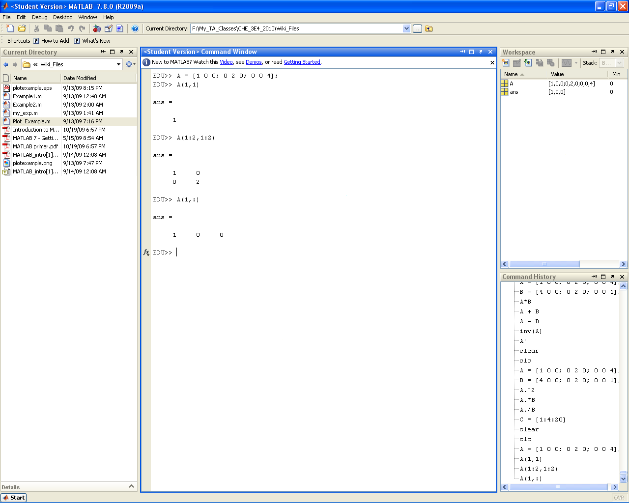
To access a value within a matrix we use the curved matrix access brackets "()". Within these brackets we place the index of the element we wish to access separated by commas (ex. (#,#,...) ). Note that MATLAB starts all its matrix indices at 1 (so it is like Fortran, not C++). MATLAB is also row dominant, so the row index comes first followed by the column index, etc. (This is quizically like C++, not Fortran). To access a subset of a given matrix we use the colon operator (:). In the context of accessing submatrices we simply state "start_point:end_point" (if it makes it easier you can just see it as start_point:1:end_point). You can do this for any of the dimensions within a matrix. If a single ":" is placed in one of the matrix dimensions this translates to "get all of this dimension". Therefore if we wanted to get all the values in row 1 of a matrix, for example (i.e. all the column values of in row 1), we would use (1,:). | |||
[[File:MATLAB_sub_matrices.PNG|center|400px]] | |||
=====Concatenation===== | |||
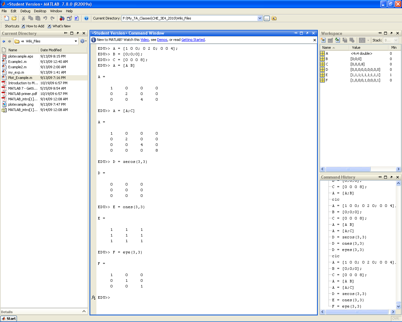
Matrices can be combined through a process called concatenation. In horizontal concatenation two matrices are joined from "left to right" (i.e. the new matrix has the same number of rows but a new number of columns equal to the sum of the columns in the two original arrays). Horizontal concatenation of two matrices is achieved through the use of the square matrix declaration brackets "[]". To concatenate the arrays simply place them in the square brackets with a space or comma between them (shown below). Naturally the two matrices being horizontally concatenated must have the same number of rows (or else MATLAB will spit out an error). Vertical concatenation follows the same logic as horizontal concatenation but combines matrices "top to bottom". This time the new matrix has the same number of columns but a new number of rows. To accomplish vertical concatenation the arrays must be placed in a square bracket separated by a semicolon (shown below). This time the arrays must have the same number of columns for the concatenation to be successfull. | |||
[[File:MATLAB_concatenation.PNG|center|400px]] | |||
== | |||
| | |||
Latest revision as of 13:40, 24 September 2010
Introduction to the Command Line
- MATLAB IS CASE SENSITIVE!!! For example, A is not the same thing as a. This is very important when working with variable and function names.
doc function_name
Brings up information on any built-in MATLAB function (i.e. it accesses the help directory entry).
| Before | After |
|---|---|
edit
Opens the text editor
| Before | After |
|---|---|
clc
Clears the screen
| Before | After |
|---|---|
clear
Clears the variables from the workspace (and from memory)
| Before | After |
|---|---|
Built in Functions
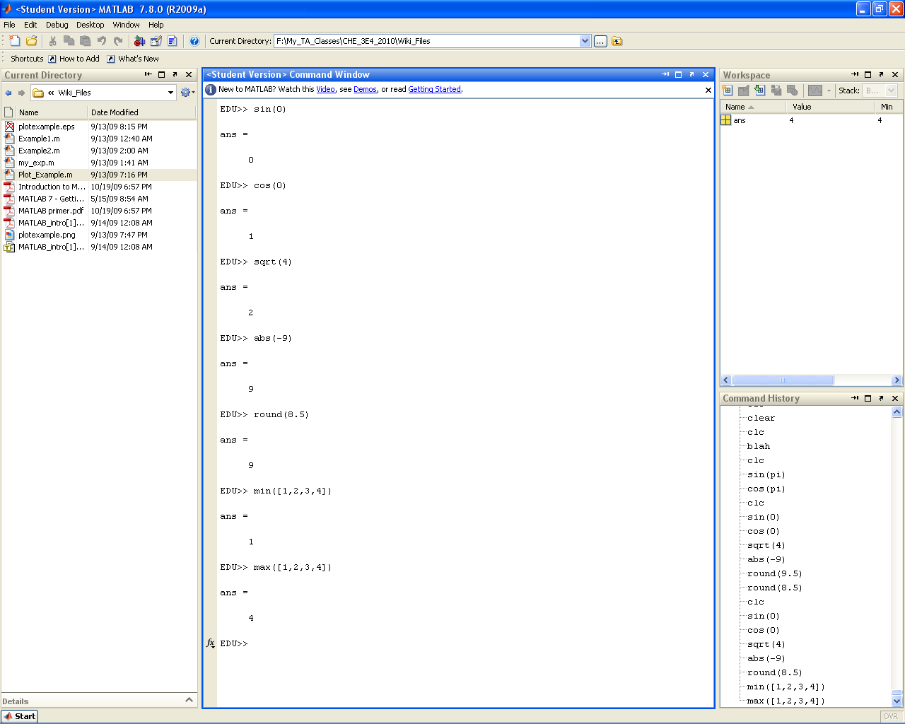
MATLAB has an array of simple built in functions. Basically all of the rudimentary calculation types that you can think of (sin,cos,exp,etc.) have a built in MATLAB function that may be called at the command line and coded into a script or function file (as the need arises). A few examples are shown in the screenshot below.
Built in Constants
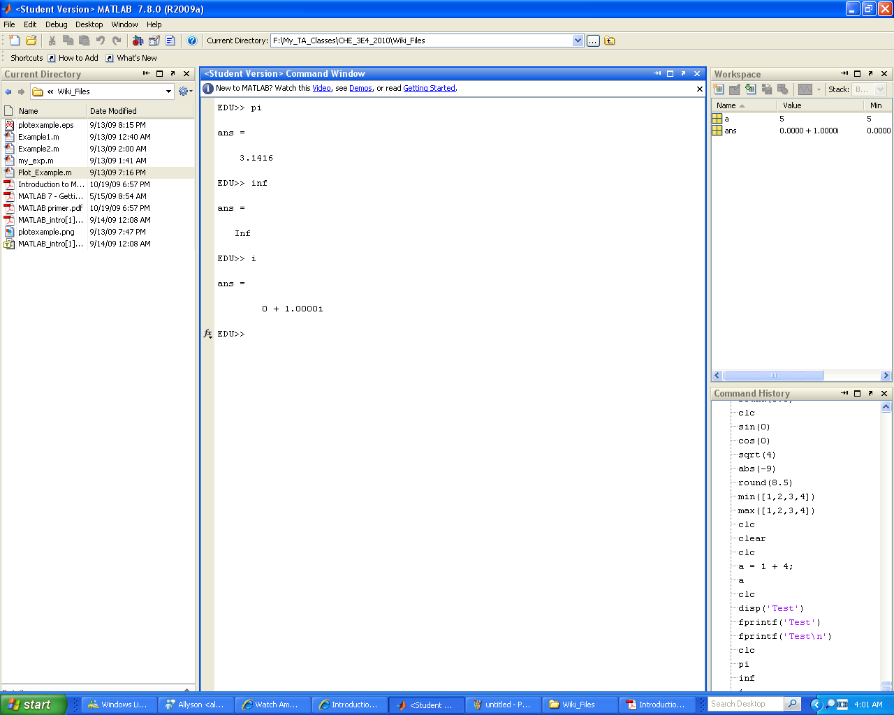
MATLAB also has predefined variables for fundamental constants (ex. pi, Inf, i). Be wary though, as these can be easily overwritten by the user. As a rule of thumb try not to name your variables after any fundamental mathematical constant.
fprintf() and disp()
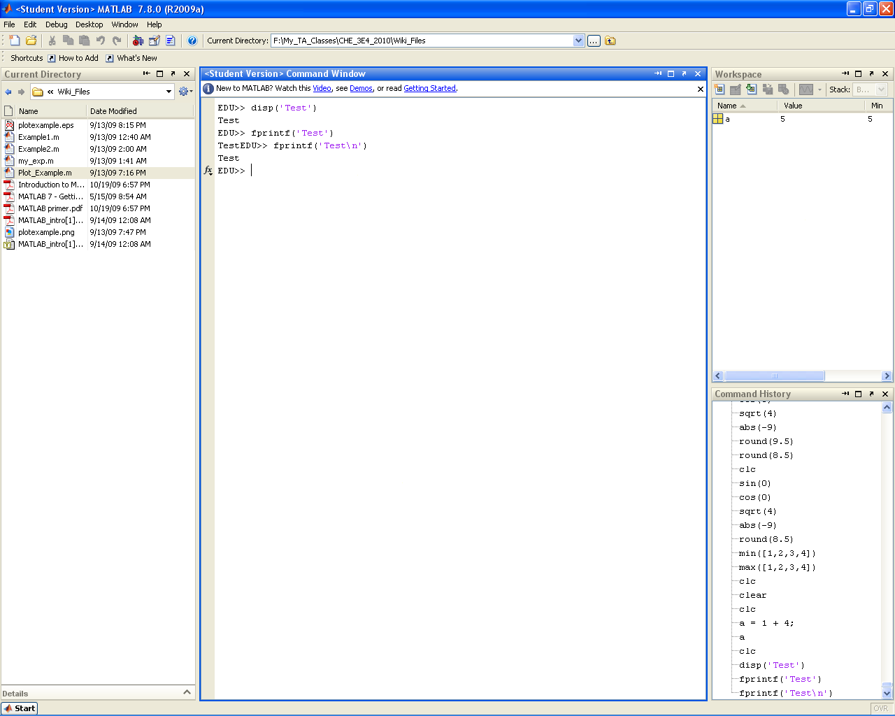
fprintf() and disp() provide a means of printing text to the command window. While obviously not useful at the command line (as the example below shows), these statements will become useful when you begin writing your own scripts and functions (either as a means of displaying intermediate results or as a means of tracking down bugs). disp() is a simple display function that prints arrays or strings directly to the command window. fprintf() is a more robust function that allows formatting of the string to be printed as well as output specification (for use in printing to files). The default output is set to the command window.
Semicolon
Placing a semicolon at the end of a line of code will suppress any output produced by that line. This (along with fprintf() and break points) can help in debugging code. Unless you are debugging it is good practice to end all lines of code with a semi-colon to avoid a bunch of garbage intermediate values being printed out at the command line.
Variables
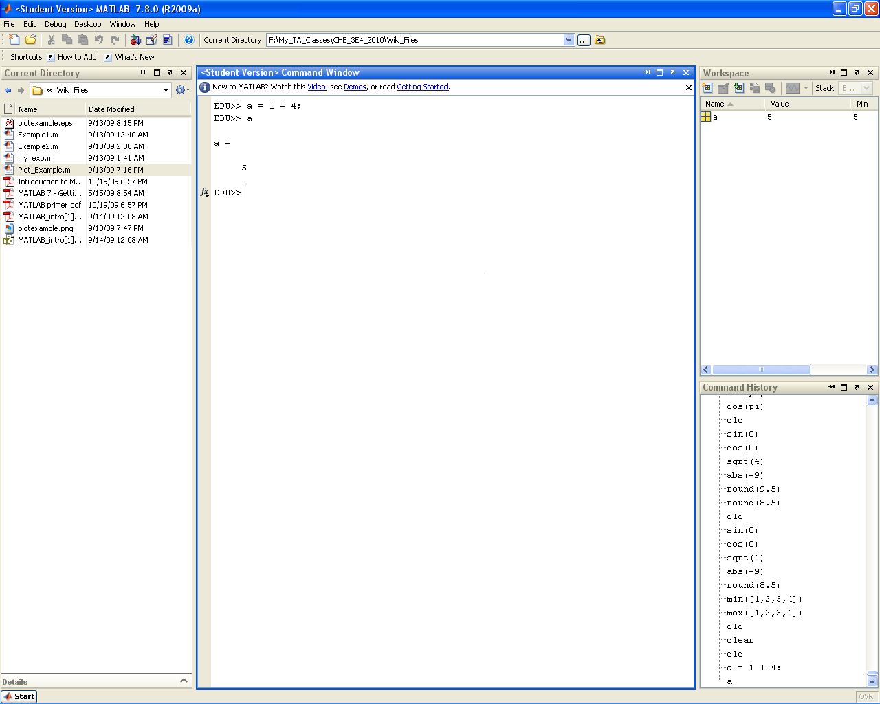
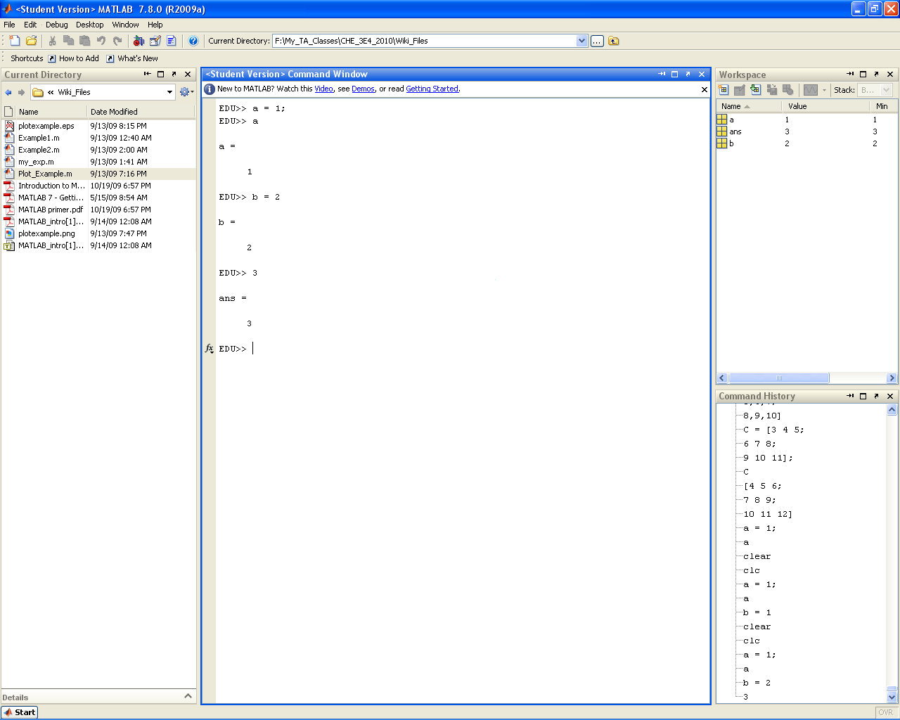
Variables declared in MATLAB are essentially 1x1 matrices. To declare a variable in MATLAB all you need to do is specify the name of the variable and then set it to a value using the "=" operator (shown below). This is the same for both MATLAB code and the command line. Note below that if you place a semi-colon after the variable declaration then the variable's value is not reprinted (the opposite is also true). Also note that if a variable is not declared for a value then the default ans variable is assigned to it. Please note that there is only one ans variable. So as soon as another undeclared value shows up the previous value will be lost. Therefore it is always a good idea to give every variable a name (to avoid plenty of headaches in the debugging stage). Also note that ans does not discriminate between variables and larger matrices, so any new undeclared variable or matrix will reassign the value of ans.
Matrices
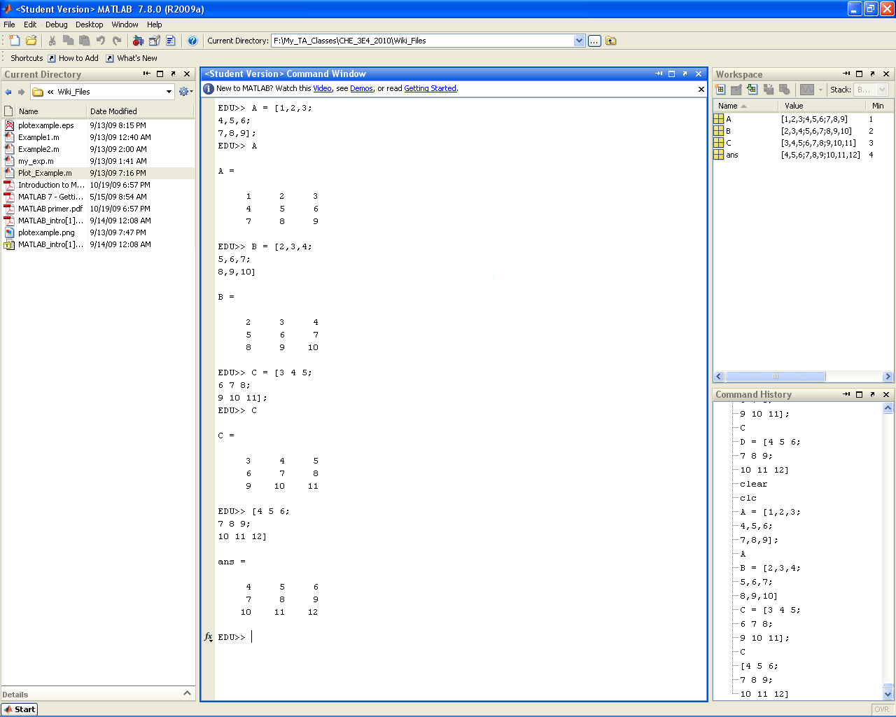
Matrices are arrays of values. To declare a matrix in MATLAB all one needs to do is use the "[]" matrix declaration brackets. Within a matrix declaration, the individual row elements are separated by a "," or a blank space (" ") and the rows are separated by a semicolon (thus it is possible to declare a matrix as it would appear on paper...). However, always remember that it is not a requirement to declare each new row on a separate line. As long as the semicolon is there, MATLAB will interpret it as the start of a new row. Note that matrices in MATLAB are declared in row dominant order (similar to C++). That is the first index refers to the row number, the second to the column number, etc. The Accessing Submatrices section below will outline how to access elements within a matrix. Also note that it is possible to create special types of "ordered" matrices using the colon (:) operator (shown in the Dot and Colon Operator section).
Matrix Operations
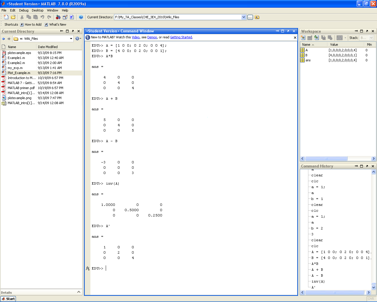
MATLAB follows all basic linear algebra rules (obviously :P). That is to say that when you add or subtract two matrices it is done on an element by element basis, while multiplication is done one a row by column basis and division performs the reverse of this operation. Note however that if you add a "." in front of a *,/, or ^ then the operation is performed on an element by element basis. Obviously adding a dot in front of a + or - would not do anything extra (and actually results in a compilation error).
Dot and Colon Operator
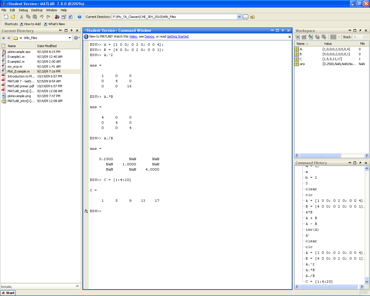
If you add a "." in front of a *,/, or ^ then the operation is performed on an element by element basis. Obviously adding a dot in front of a + or - would not do anything extra (and actually results in a compilation error). Another usefule operator is the colon operator (:). As will be seen in the next section, the colon operator is instrumental in accessing subsections within a given matrix. However, it is also used in declaring ordered sequences (both in declaring a vector with a known pattern and in declaring the pattern of a for loop. The syntax for using the colon operator to declare an ordered vector is "[start_point:step_size:end_point]". MATLAB will take this code and create a vector that starts at "start_point" and moves up incrementally by "step_size" until it is either equal to or less than "end_point" by a value less than "step_size". This is to say that the sequence will never exceed "end_point". Therefore if a "step_size" was chosen that does not exactly land on "end_point", MATLAB will fall short rather than fall over.
Accessing Submatrices
To access a value within a matrix we use the curved matrix access brackets "()". Within these brackets we place the index of the element we wish to access separated by commas (ex. (#,#,...) ). Note that MATLAB starts all its matrix indices at 1 (so it is like Fortran, not C++). MATLAB is also row dominant, so the row index comes first followed by the column index, etc. (This is quizically like C++, not Fortran). To access a subset of a given matrix we use the colon operator (:). In the context of accessing submatrices we simply state "start_point:end_point" (if it makes it easier you can just see it as start_point:1:end_point). You can do this for any of the dimensions within a matrix. If a single ":" is placed in one of the matrix dimensions this translates to "get all of this dimension". Therefore if we wanted to get all the values in row 1 of a matrix, for example (i.e. all the column values of in row 1), we would use (1,:).
Concatenation
Matrices can be combined through a process called concatenation. In horizontal concatenation two matrices are joined from "left to right" (i.e. the new matrix has the same number of rows but a new number of columns equal to the sum of the columns in the two original arrays). Horizontal concatenation of two matrices is achieved through the use of the square matrix declaration brackets "[]". To concatenate the arrays simply place them in the square brackets with a space or comma between them (shown below). Naturally the two matrices being horizontally concatenated must have the same number of rows (or else MATLAB will spit out an error). Vertical concatenation follows the same logic as horizontal concatenation but combines matrices "top to bottom". This time the new matrix has the same number of columns but a new number of rows. To accomplish vertical concatenation the arrays must be placed in a square bracket separated by a semicolon (shown below). This time the arrays must have the same number of columns for the concatenation to be successfull.
