Software tutorial/My first program
In this part of the tutorial you are required to create a plot with 10 points (a vector), consisting of the numbers
| MATLAB | Python |
|---|---|
|
There are several ways we can create our vector >> x = [0 2 4 6 8 10 12 14 16 18];
>> x = [0, 2, 4, 6, 8, 10, 12, 14, 16, 18];
>> x = linspace(0, 18, 10); % easiest method
>> x
x =
0 2 4 6 8 10 12 14 16 18
Now create the corresponding >> y = (x-8).^2 - 40;
>> y
y =
24 -4 -24 -36 -40 -36 -24 -4 24 60
Note: that we must use .^ to calculate the exponent. If you just write ^ by itself, MATLAB will assume you want to calculate the matrix exponent, which is defined quite differently. In fact, any element-by-element calculation must use the "." notation to tell MATLAB not to use its default matrix calculations. For example, use .* for element-by-element matrix multiplication. If you are bit rusty on this concept, we recommend you read page 4 and 5 of Dr. Mhaskar's Python primer. |
There are several ways we can create our vector import numpy as np
from matlabplotlib.pylab import *
>>> x = np.array([0, 2, 4, 6, 8, 10, 12, 14, 16, 18])
>>> x = np.linspace(0, 18, 10) # easiest method
>>> x
array([ 0, 2, 4, 6, 8, 10, 12, 14, 16, 18])
Now create the corresponding >>> y = (x-8) ** 2 - 40
>>> y
array([ 24., -4., -24., -36., -40., -36., -24., -4., 24., 60.])
We raise a variable to a power using the ** notation; the ^ operator means something else in Python. |
Key difference
- In MATLAB, everything is a matrix calculation, by default.
- In Python's NumPy library (numpy), everything is an element-by-element calculation, by default.
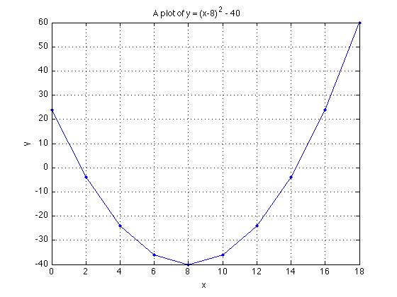
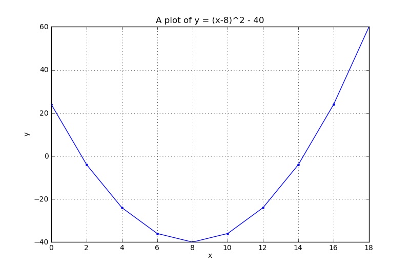
Finally, we are ready to plot these
| MATLAB | Python |
|---|---|
plot(x, y, '.-')
grid on
xlabel('x')
ylabel('y')
title('A plot of y = (x-8)^2 - 40')
|
plot(x, y, '.-')
grid('on')  # <--- it is a function in Python, so add ()
xlabel('x')
ylabel('y')
title('A plot of y = (x-8)^2 - 40')
|

