Introduction

MATLAB	Python
MATLAB (MATrix LABoratory) is a high level computer language/ interactive software package developed and distributed by MathWorks™. Matlab was first developed in the 1970s by Cleve Molar. Cleve was later joined by John N. Little and Steve Bangert and the three went on to found MathWorks™. MATLAB excels at performing matrix operations and can handle large data sets (stored as matrices) very easily. MATLAB was originally designed as a user friendly interface for LINPACK and EISPACK and so was intended for linear algebra application. Since then MATLAB has greatly expanded it's core abilities to encompass a large array of graphic and numeric applications. These core abilities may in turn be expanded further through the addition of specialized "tool boxes".	From Wikipedia: Python is a high-level programming language whose design philosophy emphasizes code readability. Python aims to combine "remarkable power with very clear syntax", and its standard library of built-in functions is large and comprehensive. We will use the NumPy and SciPy modules (the equivalent of a MATLAB toolbox), to provide scientific computing capabilities to Python. These modules, like MATLAB, allow you to handle large data arrays with little effort. They provide all the tools we require for this course. We will also use the matplotlib module, which provides Python with plotting capabilities similar to MATLAB.

Access / Installation

MATLAB	Python
MATLAB is installed on all computers in the John Hodgins Engineering Student Technology Centre (JHE 233A / 234) as well as the Burke Science Building Labs (BSB 241 / 242 / 244 / 249). The most up to date release of MATLAB is version R2010b. While there are some backward compatibility issues when it comes to older versions of MATLAB, for the level of code that will be encountered in this class students should not encounter issues with portability of code. A MATLAB/SIMULINK student package (version R2010A, good for Windows, Mac, and Linux) is available at the University Book Store for $112.95 (for those students who would like a copy of MATLAB on their laptop or home PC). The student versions comes with the following features: MATLAB version R2010a (Everything you need to get started) Simulink (Will be useful in your control classes) Control System Toolbox Signal Processing Toolbox Signal Processing Blockset Statistics Toolbox Optimization Toolbox Symbolic Math Toolbox Image Processing Toolbox Product Demos I personally have a student copy on my home PC. It's a good buy if you have the extra cash.	Python is freely available. The latest stable version that we recommend for the course is version 2.6, because it is compatible with the external libraries that we will use. Installation instructions for Python are available on this website.

Getting started

These descriptions are specific to Windows-users. Mac and Linux users will have a similar display.

MATLAB	Python
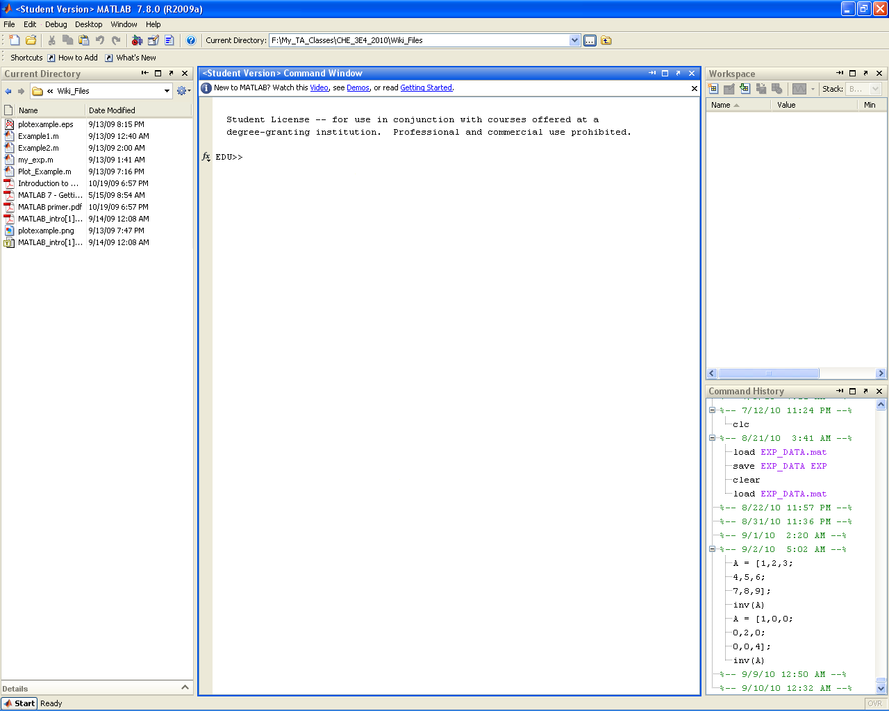
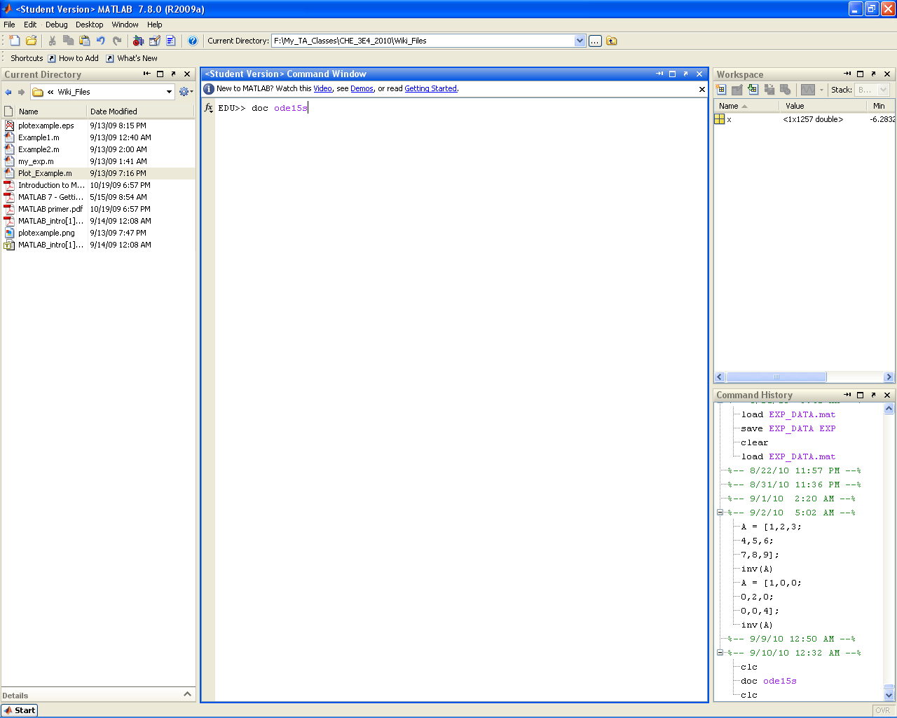
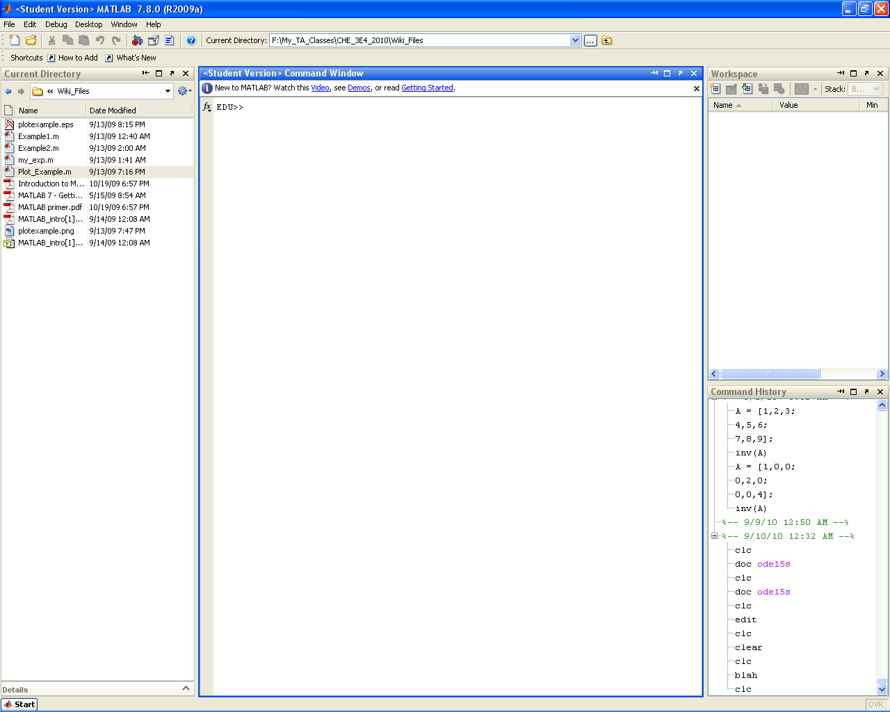
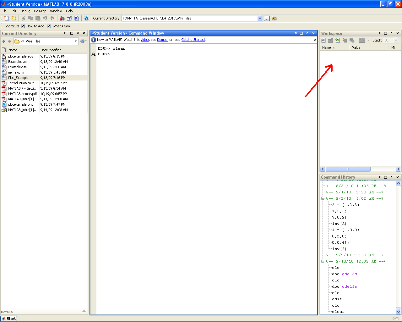
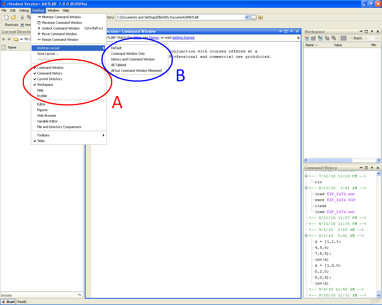
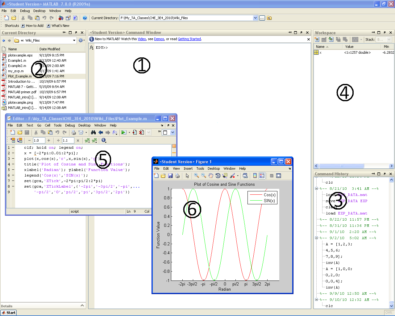
When you launch MATLAB the following window will open: Do not worry if MATLAB does not open exactly like this. You can easily modify what windows are visible through the Desktop drop down menu. You can select the windows you want either by toggling them individually (Region A) or by selecting a template (Region B). Selecting the default template should give you the window layout you saw above. The core MATLAB setup has 6 main sections of interest that you will become very familiar with by the end of this course: 1. 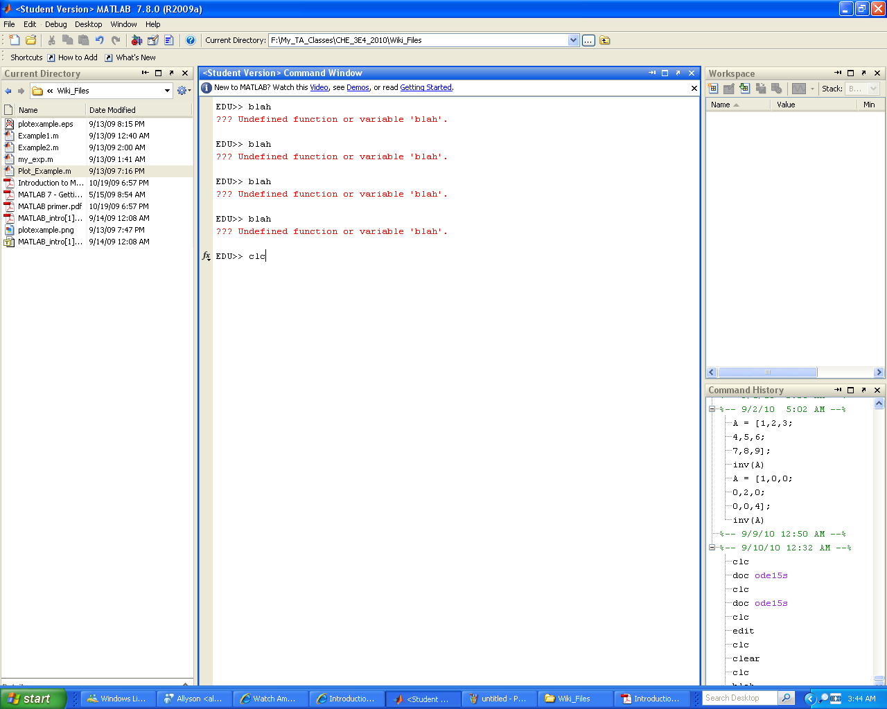Command Window The command window (or "command line") provides your main means of interacting with the MATLAB software. The command line allows you to enter simple codes that are processed immediately. All program outputs also appear in the command window. While it is technically possible to write an entire program at the command line, this is not recommended. For true programs, scripts and functions will be used. 2. Current Directory The "current directory" panel lists all of the files (MATLAB or other) that are located in the directory MATLAB is currently accessing. This directory may be changed via the drop down address bar at the top of the main program window. For a program to run properly, ALL CODES required must be in the same directory (for example, if you write a main script file that calls a separate function file, both files must be in the same directory). 3. Command History The command history records all commands entered in the command window (for possible future reference). 4. 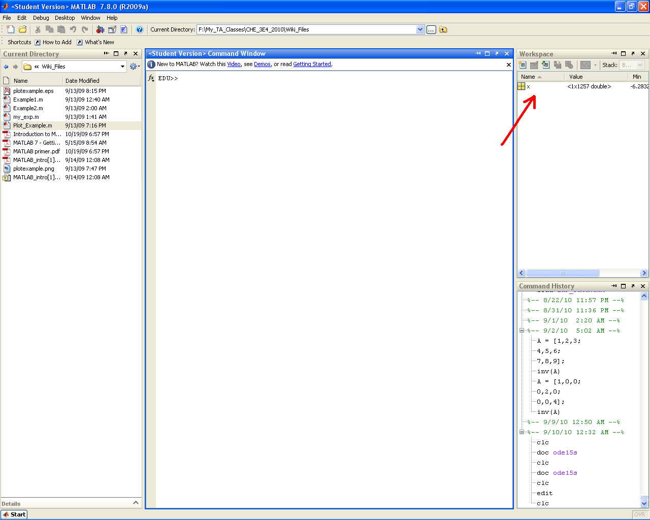Workspace The workspace lists all variables, matrices, and function handles currently being stored by MATLAB. The workspace also provides basic information on the values being stored, such as size, max, min, etc. Perhaps most useful is the ability to double click variables and matrices in the workspace to open up the Variable Editor window. The variable editor is essentially a spread sheet representation of your variables that allows for easy manipulation (especially useful for large matrices). 5. 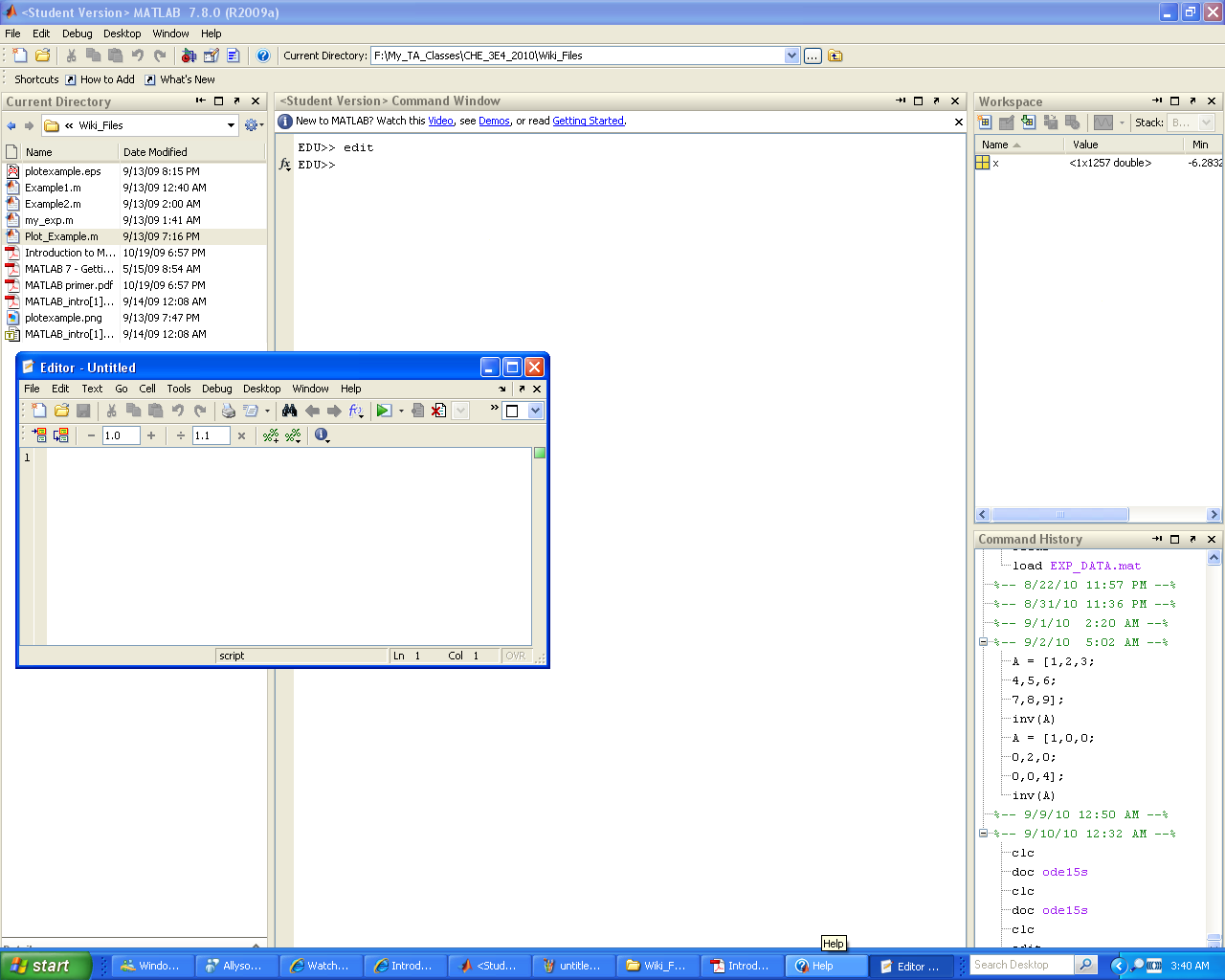Editor Window The editor window(s) does not immediately open when you launch MATLAB. The editor window is where you write scripts and function files that can be compiled and run in the command window (to be discussed in detail later). To open a new editor window you can either go to `File`>`New`>`Blank M-File`, hit Ctrl+N, type "edit" at the command line, or hit the "New M-File" icon at the top left of the main screen (it looks like the little piece of paper with the explosion in the top left corner). To open a pre-existing M-File you need to switch the current directory to the location of the file (as mentioned above) and simply double click on the M-File name in the "current directory" sidebar. 6. Plot Window When the MATLAB plot tools are used the resulting graphics are displayed in separate plot windows (more on this later).	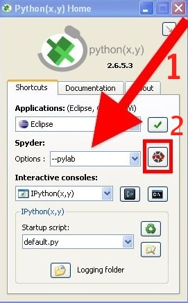When starting Python(x,y) you will be presented with the following window. Spyder (Scientific PYthon Development EnviRonment) is the name of the development environment we will be using. Select the `--pylab` option Then launch the Spyder environment. 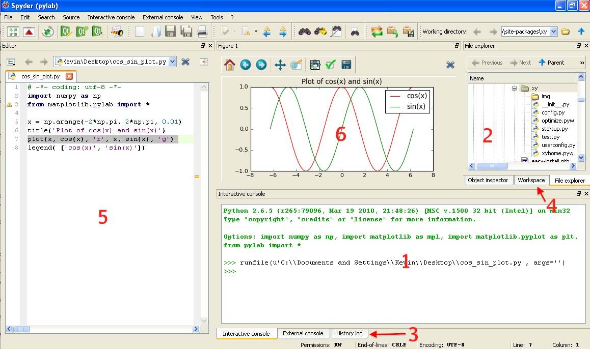Python(x,y) has a layout similar to that shown below 1. Command Window The command window is where you interact with Python. Commands entered here are processed immediately. While it is technically possible to write an entire program at the command line, this is not recommended. For true programs, you should write a script in region 5 of the software. 2. Current Directory The "current directory" panel lists all of the files that are located in the directory Python is currently accessing. This directory may be changed by navigating to a new directory and clicking on its name. 3. Command History The command history records all commands entered in the command window (for possible future reference). 4. Workspace The workspace lists all variables (e.g. vectors and matrices) currently available to you. The workspace also provides the size and "type" of variable. You can double click on a variable and change its value: e.g. edit a specific entry in a vector, in a spreadsheet-like interface. 5. Editor Window The editor window is where you write scripts and function files. After saving the file to disk, you can run it by pressing `F9` (or click on `Source` in the top menu and select `Run in interactive console`) You can have one or multiple files open at any time. 6. Plot Window Python plots are opened in new separate windows, but can be "docked" (placed) anywhere inside the main Python(x,y) window.

Your first script

In this script we will create a plot with 10 points (a vector), consisting of the numbers $x = [0, 2, 4, ... 18] $. Then we will also create a corresponding vector $y = (x-8)^2 - 40$ and plot these $ (x,y)$ points, pairwise, on a plot.

MATLAB	Python
There are several ways we can create our vector $x$ in MATLAB. x = [0 2 4 6 8 10 12 14 16 18] x = [0, 2, 4, 6, 8, 10, 12, 14, 16, 18] x = linspace(0, 18, 10) % easiest method Now create the corresponding $y$-vector using MATLAB's ability to do vector operations. We can write y = (x-8).^2 - 40 Note: that we must use `.^` to calculate the exponent. If you just write `^` by itself, MATLAB will assume you want to calculate the matrix exponent, which is defined quite differently. In fact, any element-by-element calculation must use the "." notation to tell MATLAB not to use its default matrix calculations. For example, use `.*` for element-by-element matrix multiplication.	There are several ways we can create our vector $x$ in Python. import numpy as np from matlabplotlib.pylab import * x = np.array([0, 2, 4, 6, 8, 10, 12, 14, 16, 18]) x = np.linspace(0, 18, 10) # easiest method Now create the corresponding $y$-vector: y = (x-8) 2 - 40 We raise a variable to a power using the `` notation; the `^` operator means something else in Python.

Key difference

In MATLAB, everything is a matrix calculation, by default.
In Python's NumPy library (numpy), everything is an element-by-element calculation, by default.

Introduction to the Command Line

MATLAB

MATLAB IS CASE SENSITIVE!!! For example, A is not the same thing as a. This is very important when working with variable and function names.

Common Command Line Commands and Functions

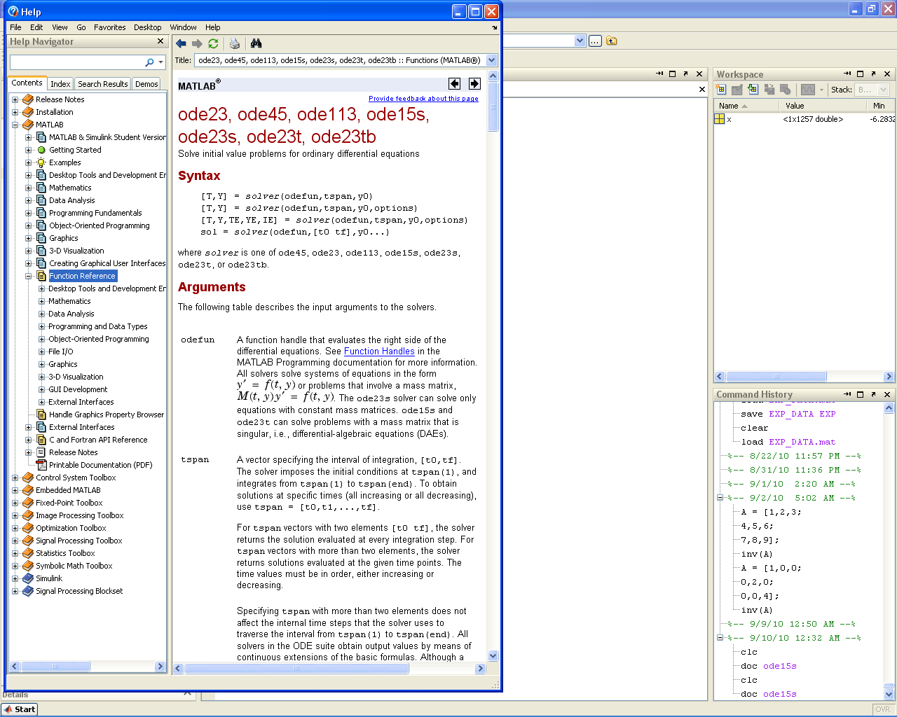
doc function_name

Brings up information on any built-in MATLAB function (i.e. it accesses the help directory entry).

Before	After

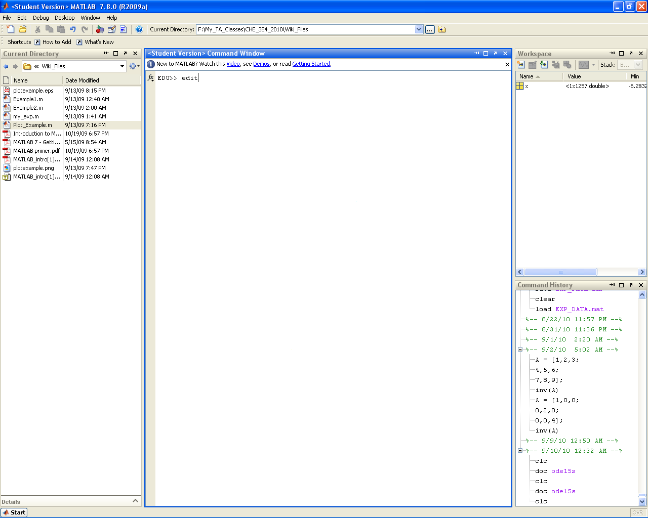
edit

Opens the text editor

Before	After

clc

Clears the screen

Before	After

clear

Clears the variables from the workspace (and from memory)

Before	After

Built in Functions

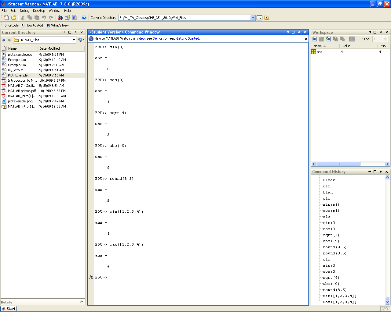
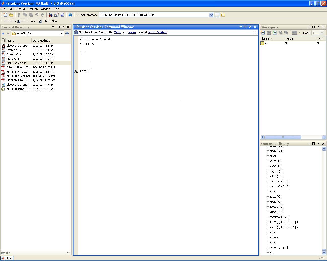
MATLAB has an array of simple built in functions. Basically all of the rudimentary calculation types that you can think of (sin,cos,exp,etc.) have a built in MATLAB function that may be called at the command line and coded into a script or function file (as the need arises). A few examples are shown in the screenshot below.

Built in Constants

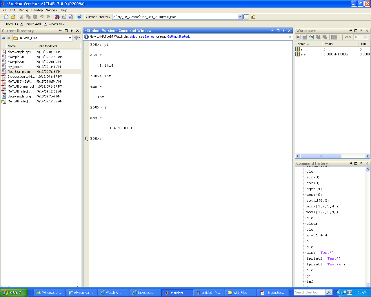
MATLAB also has predefined variables for fundamental constants (ex. pi, Inf, i). Be wary though, as these can be easily overwritten by the user. As a rule of thumb try not to name your variables after any fundamental mathematical constant.

fprintf() and disp()

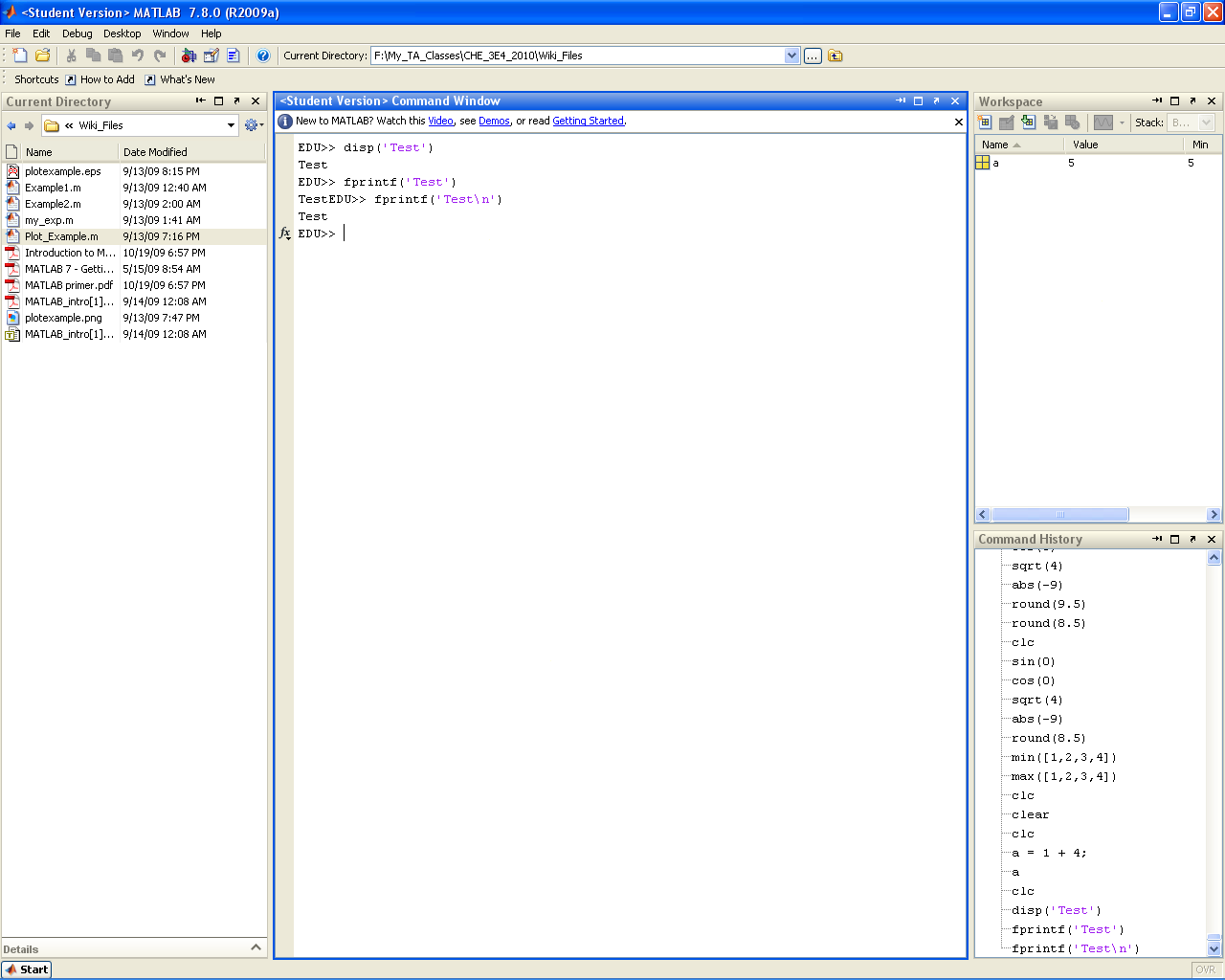
fprintf() and disp() provide a means of printing text to the command window. While obviously not useful at the command line (as the example below shows), these statements will become useful when you begin writing your own scripts and functions (either as a means of displaying intermediate results or as a means of tracking down bugs). disp() is a simple display function that prints arrays or strings directly to the command window. fprintf() is a more robust function that allows formatting of the string to be printed as well as output specification (for use in printing to files). The default output is set to the command window.

Semicolon

Placing a semicolon at the end of a line of code will suppress any output produced by that line. This (along with fprintf() and break points) can help in debugging code. Unless you are debugging it is good practice to end all lines of code with a semi-colon to avoid a bunch of garbage intermediate values being printed out at the command line.

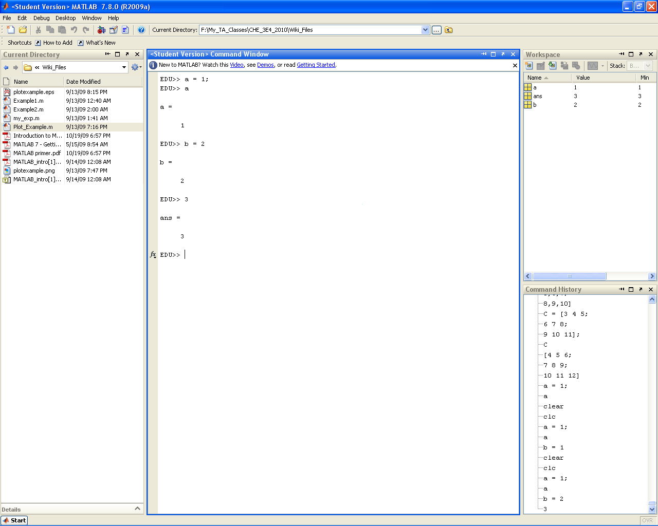
Variables

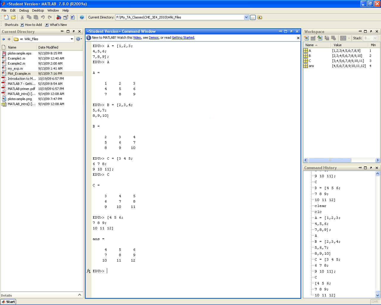
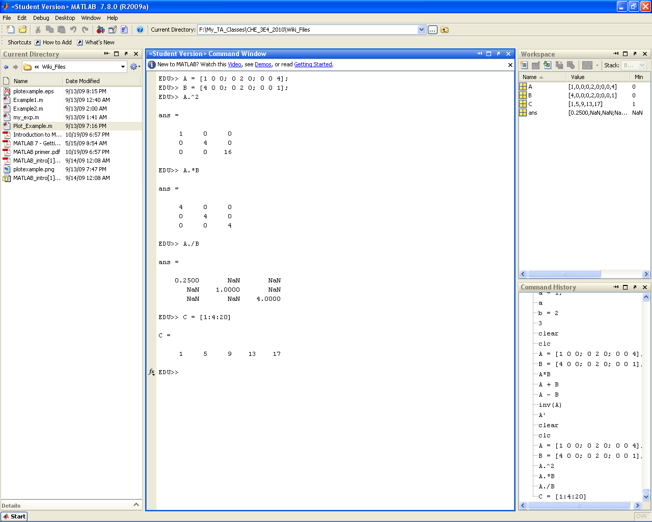
Matrices

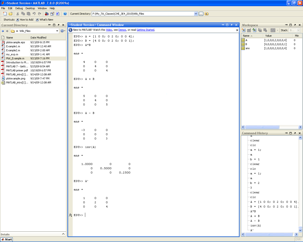
Matrix Operations

Dot and Colon Operator

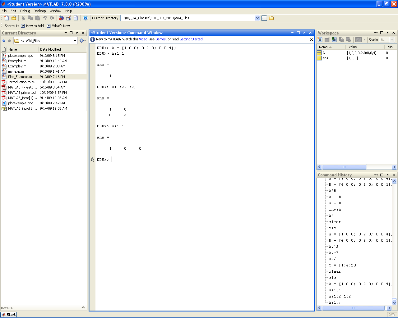
Accessing Submatrices

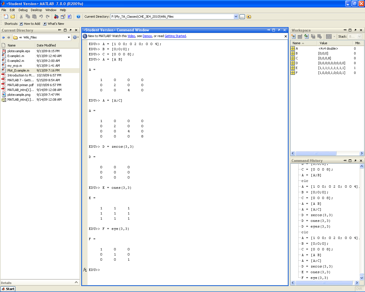
Concatenation

Python