Software tutorial/Extracting information from a linear model in R
<rst>
<rst-options: 'toc' = False/>
<rst-options: 'reset-figures' = False/>
Getting the model coefficients
Once the model is built, :math:`y = b_0 + b_1 x + e`, you can see that the :math:`b_0` coefficient is 1.50 and :math:`b_1` coefficient is 0.70 from the ``summary(...)`` output. What if you want the coefficients directly?
.. code-block:: s
x <- c(1, 2, 3, 4, 5) y <- c(2, 3, 4, 4, 5) model <- lm(y~x)
model.cf <- coef(model) model.cf # (Intercept) x # 1.5 0.7 b.0 <- model.cf[1] b.1 <- model.cf[2]
# Use the model to calculate predictions for some new x-values # (although we show a better way to do this further down!) x.new = c(1.5, 2, 4) y.new = b.0 + b.1 * x.new y.new # [1] 2.55 2.90 4.30
Getting the model's residuals, standard error, and predicted values
The linear model object, ``model``, in this example, contains several attributes (sub-entries) that you can access. For example, the residuals:
.. code-block:: s
model$residuals # 1 2 3 4 5 # -2.000000e-01 1.000000e-01 4.000000e-01 -3.000000e-01 2.289835e-16 There are several other attributes; use the ``names(...)`` function to get a complete list of attributes. .. code-block:: s names(model) # [1] "coefficients" "residuals" "effects" "rank" "fitted.values" "assign" # [7] "qr" "df.residual" "xlevels" "call" "terms" "model" Another example is ``model$df.residual``, which will give you the number of degrees of freedom associated with the residuals (3 in this case).
However, there is a preferred way to access most of the common attributes. These are called accessor functions.
============================== =========================== =======================
Item type Sub-entry in linear model Preferred way to access it
============================== =========================== =======================
Model coefficients ``model$coefficients`` ``coef(model)`` Residuals ``model$residuals`` ``residuals(model)`` Predicted outputs, :math:`\hat{y}` ``model$fitted.values`` ``fitted(model)`` ======'"`UNIQ--h-2--QINU`"'============================== =========================== ============================= .. '"`UNIQ--syntaxhighlight-00000000-QINU`"' .. .. '"`UNIQ--syntaxhighlight-00000002-QINU`"' .. .. '"`UNIQ--syntaxhighlight-00000004-QINU`"' .. Unfortunately there is no standard way to get access to the standard error (that I am aware of). This approach will work though: .. code-block:: s SE <- sqrt( sum( residuals(model)^2 ) / model$df.residual )
The above is just a direct implementation of :math:`S_E = \sqrt{\frac{\displaystyle \sum{e_i^2}}{\displaystyle n - k }}`
Checking if the residuals are normally distributed
Here's another example of the object nature of a linear model. Certain functions in R will work on these objects and do something sensible with them. For example, the ``qqPlot(...)`` function will check that the residuals are normally distributed. You :ref:`first need to install <r-installing-packages>` and load the ``car`` library though:
.. code-block:: s
library(car) qqPlot(model) # Don't be surprised by the strange plot - there are only 5 observations in the model
Calculating confidence intervals for the model parameters
We know that the confidence intervals for :math:`\beta_0` and :math:`\beta_1` are given by:
.. math::
\begin{array}{rcccl} b_0 - c_t S_E(b_0) &\leq& \beta_0 &\leq&b_0 + c_t S_E(b_0) \\ b_1 - c_t S_E(b_1) &\leq& \beta_1 &\leq& b_1 + c_t S_E(b_1) \end{array}
where the :math:`c_t` value is the critical value from the t-distribution at the particular confidence level, e.g. 95%.
.. math::
\begin{array}{rcl} S_E^2(b_0) &=& \mathcal{V}\{b_0\} = S_E^2 \left(\dfrac{1}{n} + \dfrac{\bar{\mathrm{x}}^2}{\sum_j{\left( x_j - \bar{\mathrm{x}} \right)^2}} \right)\\ S_E^2(b_1) &=& \mathcal{V}\{b_1\} = \dfrac{S_E^2}{\sum_j{\left( x_j - \bar{\mathrm{x}} \right)^2}} \end{array}
Fortunately you don't need to perform these tedious calculations by hand in R every time. Use the ``confint(...)`` function instead. Below we calculate the 99% confidence intervals for the intercept and slope. Note that the intercept CI crosses zero in this example.
.. code-block:: s
confint(model, level=0.99) # 0.5 % 99.5 % # (Intercept) -0.4372105 3.437210 # x 0.1159091 1.284091
Using a linear model with new :math:`x`-values
Other than learning more about our system (i.e. interpreting the model parameter confidence intervals), we also build models to make predictions from future :math:`x` data. We use the ``predict(model, ...)`` function in R. With no additional options, it will return the model training predictions, the same output as ``fitted(model)``.
.. code-block:: s
predict(model) # 1 2 3 4 5 # 2.2 2.9 3.6 4.3 5.0
But we must first create a prediction data set to use the model on new :math:`x` data. I'm going to create a new model for this section.
.. code-block:: s
density <- c(800, 1100, 1200, 1000, 1150) viscosity <- c(96, 73, 53, 72, 53) model <- lm(viscosity ~ density)
Now create a new data set containing 6 ``density.new`` values. The key point is that the column name in this new data frame *must be the same* one that was used to build the model (i.e. ``density``).
.. code-block:: s
density.new <- data.frame(density = c(750, 850, 950, 1050, 1150, 1250)) density.new # density # 1 750 # 2 850 # 3 950 # 4 1050 # 5 1150 # 6 1250
Now use this new data frame in the ``predict(model, ...)`` function as the ``newdata`` argument:
.. code-block:: s
y.hat.new <- predict(model, newdata=density.new) y.hat.new # 1 2 3 4 5 6 # 101.5 90.8 80.1 69.4 58.7 48.0
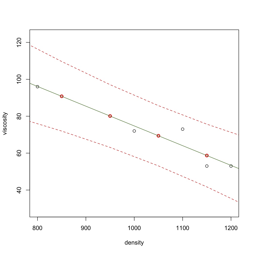
Let's visualize this: these predictions are shown in red, and the least squares line in green.
.. code-block:: s
plot(density, viscosity, ylim=range(y.hat.new)) points(density.new$density, y.hat.new, col="red", lwd=2) abline(model, col="darkgreen") </rst> [[Image:least-squares-prediction-plot.jpg|450px|center]] <rst> <rst-options: 'toc' = False/> <rst-options: 'reset-figures' = False/> Recall that the prediction interval for :math:`\hat{y}` from a new x measurement :math:`x_\text{new}` is given by: :math:`\hat{y}_i \pm c_t \sqrt{V\{\hat{y}_i\}}` where :math:`\mathcal{V}\{\hat{y}_i\} = S_E^2\left(1 + \dfrac{1}{n} + \dfrac{(x_i - \bar{\mathrm{x}})^2}{\sum_j{\left( x_j - \bar{\mathrm{x}} \right)^2}}\right)` Again, this is tedious to calculate by hand. For example, to get the 90% prediction intervals: .. code-block:: s y.hat.new.PI <- predict(model, newdata=density.new, interval="p", level=0.90) y.hat.new.PI # fit lwr upr # 1 101.5 79.90412 123.09588 # 2 90.8 71.94957 109.65043 # 3 80.1 63.10846 97.09154 # 4 69.4 53.07505 85.72495 # 5 58.7 41.70846 75.69154 # 6 48.0 29.14957 66.85043 The lower and upper bounds are the last two columns, while the fitted (prediction) values are in the first column. So now add the prediction interval to our visualization. Notice the expected quadratic curvature. .. code-block:: s plot(density, viscosity, ylim=range(y.hat.new.PI)) points(density.new$density, y.hat.new.PI[,1], col="red", lwd=2) abline(model, col="darkgreen") lines(density.new$density, y.hat.new.PI[,2], col="red", lty=2) lines(density.new$density, y.hat.new.PI[,3], col="red", lty=2)
</rst>
