Difference between revisions of "Assignment 7 - 2013"
Jump to navigation
Jump to search
Kevin Dunn (talk | contribs) (Created page with "{{OtherSidebar | due_dates = 15 November 2013, at class | dates_alt_text = Due date(s) | questions_PDF = 4N4-2013-Assignment-7.pdf | questions_link = | questions_text_alt = As...") |
Kevin Dunn (talk | contribs) |
||
| (4 intermediate revisions by the same user not shown) | |||
| Line 10: | Line 10: | ||
| other_instructions = ''Tutorial date: 11 November 2013'' | | other_instructions = ''Tutorial date: 11 November 2013'' | ||
}} | }} | ||
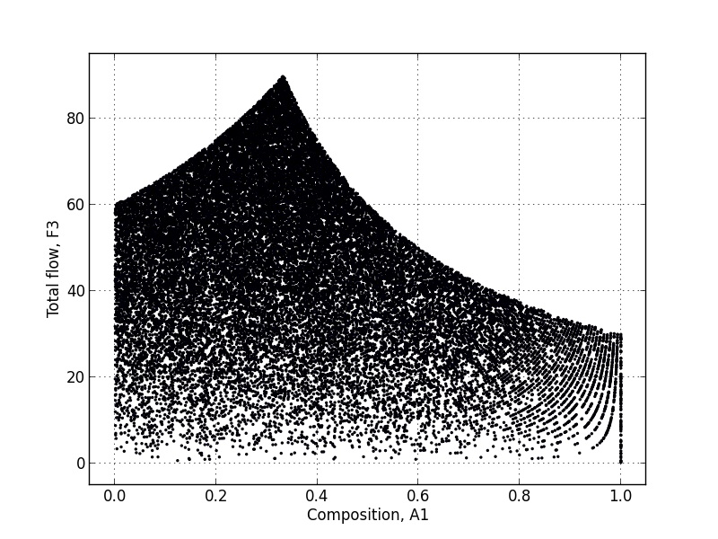
A brute force approach to get the operating window for a very simple system is to "operate" (simulate) the process at a variety of combinations of points. This is what the code does below. | |||
More challenging simulations (e.g. in Aspen) would be done by picking only a few selected points to confirm your expectations on the process, and to simulate regions in the window where you are unable to predict the result. | |||
[[Image:operating-window-assignment-7-4N4-2013.jpg]] | |||
<syntaxhighlight lang="python"> | |||
import numpy as np | |||
from matplotlib import pyplot | |||
N=100 | |||
for Fs in np.arange(0, 60.00001,0.2): # The process can operate between 0 and 100% open for Fs | |||
for Fa in np.random.uniform(0,30.00001,N): # The process can operate between 0 and 100% open for Fa | |||
flow = Fa + Fs | |||
composition = Fa/(flow + 1E-9) | |||
pyplot.scatter(composition, flow, s=2) | |||
# then plot the data as a dot; every dot represents a valid operating point | |||
pyplot.grid() | |||
pyplot.xlabel('Composition, A1') | |||
pyplot.ylabel('Total flow, F3') | |||
pyplot.xlim([-0.05, 1.05]) | |||
pyplot.ylim([-5, 95]) | |||
pyplot.savefig('operating-window-assignment-7-4N4-2013.png') | |||
pyplot.show() | |||
</syntaxhighlight> | |||
Latest revision as of 14:32, 22 November 2013
| Due date(s): | 15 November 2013, at class |
| Assignment questions | |
| Other instructions | Tutorial date: 11 November 2013 |
A brute force approach to get the operating window for a very simple system is to "operate" (simulate) the process at a variety of combinations of points. This is what the code does below.
More challenging simulations (e.g. in Aspen) would be done by picking only a few selected points to confirm your expectations on the process, and to simulate regions in the window where you are unable to predict the result.
import numpy as np
from matplotlib import pyplot

N=100
for Fs in np.arange(0, 60.00001,0.2):			# The process can operate between 0 and 100% open for Fs
    for Fa in np.random.uniform(0,30.00001,N):	# The process can operate between 0 and 100% open for Fa
        flow = Fa + Fs
        composition = Fa/(flow + 1E-9)
        pyplot.scatter(composition, flow, s=2)

# then plot the data as a dot; every dot represents a valid operating point
pyplot.grid()
pyplot.xlabel('Composition, A1')
pyplot.ylabel('Total flow, F3')
pyplot.xlim([-0.05, 1.05])
pyplot.ylim([-5, 95])
pyplot.savefig('operating-window-assignment-7-4N4-2013.png')
pyplot.show()
