Difference between revisions of "Principal Component Analysis"
Jump to navigation
Jump to search
Kevin Dunn (talk | contribs) m |
Kevin Dunn (talk | contribs) m (→Update) |
||
Line 76: | Line 76: | ||
This illustration should help better explain what I trying to get across in class 2B | This illustration should help better explain what I trying to get across in class 2B | ||
* \(p_1\) and \(p_2\) are the unit vectors for components 1 and 2. | * \(p_1\) and \(p_2\) are the unit vectors for components 1 and 2. | ||
* \( \mathbf{x}_i \) is a row of data from matrix \( \mathbf{X}\). | * \( \mathbf{x}_i \) is a row of data from matrix \( \mathbf{X}\). | ||
Line 87: | Line 83: | ||
* \(\mathbf{e}_{i,2} \) = is the prediction error '''''vector''''' because the prediction \(\hat{\mathbf{x}}_{i} \) is not exact: the data point \( \mathbf{x}_i \) lies above the plane defined by \(p_1\) and \(p_2\). This \(e_{i,2} \) is the residual distance after using 2 components. | * \(\mathbf{e}_{i,2} \) = is the prediction error '''''vector''''' because the prediction \(\hat{\mathbf{x}}_{i} \) is not exact: the data point \( \mathbf{x}_i \) lies above the plane defined by \(p_1\) and \(p_2\). This \(e_{i,2} \) is the residual distance after using 2 components. | ||
* \( \mathbf{x}_i = \hat{\mathbf{x}}_{i} + \mathbf{e}_{i,2} \) is also a vector summation and shows how \( \mathbf{x}_i \) is broken down into two parts: \(\hat{\mathbf{x}}_{i} \) is a vector on the plane, while \( \mathbf{e}_{i,2} \) is the vector perpendicular to the plane. | * \( \mathbf{x}_i = \hat{\mathbf{x}}_{i} + \mathbf{e}_{i,2} \) is also a vector summation and shows how \( \mathbf{x}_i \) is broken down into two parts: \(\hat{\mathbf{x}}_{i} \) is a vector on the plane, while \( \mathbf{e}_{i,2} \) is the vector perpendicular to the plane. | ||
| | [[Image:geometric-interpretation-of-PCA-xhat-residuals.png|700px]] |
Revision as of 02:32, 19 September 2011
| ||||||
Video timing |
||||||
| ||||||
| ||||||
Video timing |
||||||
| ||||||
| ||||||
Video timing |
||||||
|
Class notes
<pdfreflow> class_date = 16 September 2011 [1.65 Mb] button_label = Create my projector slides! show_page_layout = 1 show_frame_option = 1 pdf_file = lvm-class-2.pdf </pdfreflow>
- Also download these 3 CSV files and bring them on your computer:
- Peas dataset: http://datasets.connectmv.com/info/peas
- Food texture dataset: http://datasets.connectmv.com/info/food-texture
- Food consumption dataset: http://datasets.connectmv.com/info/food-consumption
Class preparation
Class 2 (16 September)
- Reading for class 2
- Linear algebra topics you should be familiar with before class 2:
- matrix multiplication
- that matrix multiplication of a vector by a matrix is a transformation from one coordinate system to another (we will review this in class)
- linear combinations (read the first section of that website: we will review this in class)
- the dot product of 2 vectors, and that they are related by the cosine of the angle between them (see the geometric interpretation section)
Class 3 (23 September)
- Least squares:
- what is the objective function of least squares
- how to calculate the two regression coefficients \(b_0\) and \(b_1\) for \(y = b_0 + b_1x + e\)
- understand that the residuals in least squares are orthogonal to \(x\)
- Some optimization theory:
- how an optimization problem is written with equality constraints
- the Lagrange multiplier principle for solving simple, equality constrained optimization problems
- Reading on cross validation
Update
This illustration should help better explain what I trying to get across in class 2B
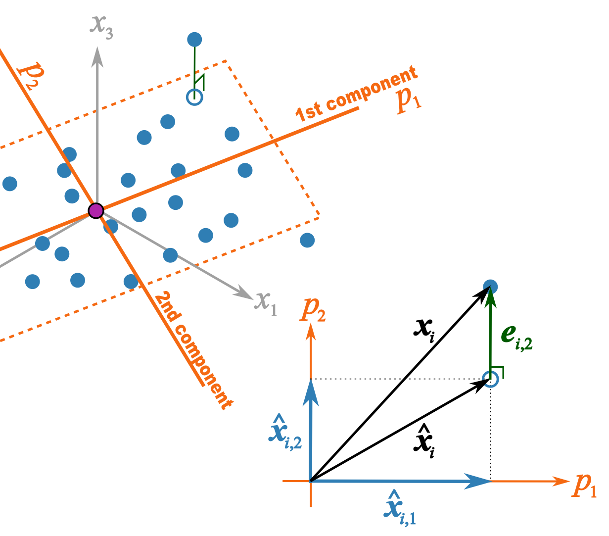
- \(p_1\) and \(p_2\) are the unit vectors for components 1 and 2.
- \( \mathbf{x}_i \) is a row of data from matrix \( \mathbf{X}\).
- \(\hat{\mathbf{x}}_{i,1} = t_{i,1}p_1\) = the best prediction of \( \mathbf{x}_i \) using only the first component.
- \(\hat{\mathbf{x}}_{i,2} = t_{i,2}p_2\) = the improvement we add after the first component to better predict \( \mathbf{x}_i \).
- \(\hat{\mathbf{x}}_{i} = \hat{\mathbf{x}}_{i,1} + \hat{\mathbf{x}}_{i,2} \) = is the total prediction of \( \mathbf{x}_i \) using 2 components and is the open blue point lying on the plane defined by \(p_1\) and \(p_2\). Notice that this is just the vector summation of \( \hat{\mathbf{x}}_{i,1}\) and \( \hat{\mathbf{x}}_{i,2}\).
- \(\mathbf{e}_{i,2} \) = is the prediction error vector because the prediction \(\hat{\mathbf{x}}_{i} \) is not exact: the data point \( \mathbf{x}_i \) lies above the plane defined by \(p_1\) and \(p_2\). This \(e_{i,2} \) is the residual distance after using 2 components.
- \( \mathbf{x}_i = \hat{\mathbf{x}}_{i} + \mathbf{e}_{i,2} \) is also a vector summation and shows how \( \mathbf{x}_i \) is broken down into two parts: \(\hat{\mathbf{x}}_{i} \) is a vector on the plane, while \( \mathbf{e}_{i,2} \) is the vector perpendicular to the plane.