Software tutorial/Creating and saving plots
Creating a plot
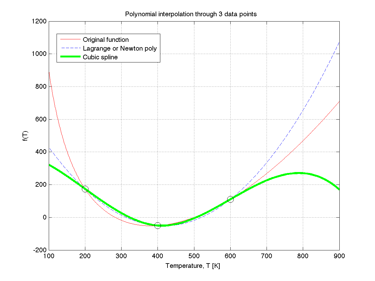
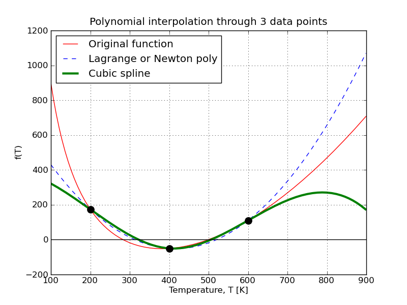
In this tutorial I will show how this plot, which we used in class, was created:
| MATLAB | Python |
|---|---|
There are several libraries to create plots in Python, but one of the most well-developed and supported libraries is matplotlib; another reason to use this library is that its syntax is intentionally similar to MATLAB's.
Plots in MATLAB and Python use an approach where you add successive elements to your graph. You start by plotting a line, then you may superimpose another line, optionally add some points, add a grid, title, labels and legend. Once completed, you can save your plot and add it to a document, website, or print it.
Use the code below, together with the comments, to understand how the plot was constructed.
| MATLAB | Python |
|---|---|
|
Put this code in a file called lagrange.m function y = lagrange(x, xx, yy)
% Returns the p_2(x) Lagrange polynomial for 3 points.
% >>> y = lagrange(x, xx, yy)
%
% INPUTS:
% x: New value(s) of x at which to evaluate the
% polynomial. Can be a scalar, or a vector.
% xx: A vector of x-values, 3 data points
% yy: A vector of y-values, 3 data points
% Calculates the Lagrange polynomial
y = yy(1)*l1(x, xx) + yy(2)*l2(x, xx) + yy(3)*l3(x, xx);
% Sub-functions used inside the ``lagrange`` function
function y = l1(x, xx)
y = (x-xx(2)).*(x-xx(3)) ./ ( (xx(1)-xx(2))*(xx(1)-xx(3)));
function y = l2(x, xx)
y = (x-xx(1)).*(x-xx(3)) ./ ( (xx(2)-xx(1))*(xx(2)-xx(3)));
function y = l3(x, xx)
y = (x-xx(1)).*(x-xx(2)) ./ ( (xx(3)-xx(1))*(xx(3)-xx(2)));
Put this code in a file called cubic_spline_3pts.m function y = cubic_spline_3pts(x, xx)
% Evaluates the cubic spline that was built from 3 nodes.
% Can be extended to splines built from more data nodes.
% >>> y = cubic_spline_3pts(x, xx)
%
% INPUTS:
% x: New value(s) of x at which to evaluate the
% polynomial. Can be a scalar, or a vector.
% xx: The x-value of the nodes at which the cubic
% spline was built.
% Since ``x`` can be a vector, we must iterate through the vector
% and evalute the polynomial at each entry in ``x``. Use the
% ``enumerate`` function in Python.
y = zeros(size(x));
k = 1;
for val = x
% Find which polynomial to use, based on the value of ``val``:
% sp stack of a sequence: if-else if-else if- ... -else if-else
if val < xx(2)
y(k) = s1(val);
%else if val < xx(...)
% etc
else
y(k) = s2(val);
end
k = k + 1;
end
function y = s1(x)
% Spline connecting nodes 1 and 2
coef = [1.2e-05, -7.2e-03, -1.6e-01, 3.98e+02];
% Note: polynomial coefficients in MATLAB go from the
% highest power to the lower power.
y = polyval(coef, x);
function y = s2(x)
% Spline connecting nodes 2 and 3
coef = [-1.2e-05, 2.16e-02, -1.168e+01, 1.934e+03];
y = polyval(coef, x);
Then put this code in another m-file (you can use any name) original_function = @(T) -24097.0-(0.26.*T)+(0.00169.*(T.^2)) ...
+ (150000.0./T) + 23505.0;
% Plot the base function
T = 100.0:1.0:900.0;
plot(T, original_function(T), 'r-')
grid('on')
% The 3 data points used
nodes = [200.0, 400.0, 600.0];
f_nodes = original_function(nodes);
% MATLAB specific: after the first plot, you must "hold" the plot
hold('on')
% Plot Lagrange polynomial: use a dashed blue line
plot(T, lagrange(T, nodes, f_nodes), 'b--')
% Cubic spline in using a thicker green
plot(T, cubic_spline_3pts(T, nodes), 'g-', 'linewidth', 3)
% Finally, add the 3 data points, as black circles
plot(nodes, f_nodes, 'ko', 'markersize', 10)
% Labels for the plot
xlabel('Temperature, T [K]')
ylabel('f(T)')
title('Polynomial interpolation through 3 data points')
legend('Original function', 'Lagrange or Newton poly', ...
'Cubic spline', 0)
% Save the plot
print('-dpng', 'polynomial_interpolation_MATLAB.png');
|
Put all this code in a py-file (you can use any name) import numpy as np
from matplotlib.pylab import *
def original_function(T):
""" Heat of reaction, as a function of temperature"""
return -24097.0-(0.26*T)+(0.00169*(T**2)) \
+ (150000.0/T) + 23505.0
def lagrange(x, xx, yy):
"""
Returns the p_2(x) Lagrange polynomial for 3 points.
>>> y = lagrange(x, xx, yy)
INPUTS:
x: New value(s) of x at which to evaluate the
polynomial. Can be a scalar, or a vector.
xx: A vector of x-values, 3 data points
yy: A vector of y-values, 3 data points
"""
# Sub-functions used inside the ``lagrange`` function
def l1(x, xx):
return (x-xx[1])*(x-xx[2]) / ( (xx[0]-xx[1])*(xx[0]-xx[2]))
def l2(x, xx):
return (x-xx[0])*(x-xx[2]) / ( (xx[1]-xx[0])*(xx[1]-xx[2]))
def l3(x, xx):
return (x-xx[0])*(x-xx[1]) / ( (xx[2]-xx[0])*(xx[2]-xx[1]))
# Calculates the Lagrange polynomial
return yy[0]*l1(x, xx) + yy[1]*l2(x, xx) + yy[2]*l3(x, xx)
def cubic_spline_3pts(x, xx):
"""
Evaluates the cubic spline that was built from 3 nodes.
Can be extended to splines built from more data nodes.
>>> y = cubic_spline_3pts(x, xx)
INPUTS:
x: New value(s) of x at which to evaluate the
polynomial. Can be a scalar, or a vector.
xx: The x-value of the nodes at which the cubic
spline was built.
"""
def s1(x):
""" Spline connecting nodes 1 and 2 """
coef = np.array([1.2e-05, -7.2e-03, -1.6e-01, 3.98e+02])
# Note: polynomial coefficients in Python go from the
# highest power to the lower power.
return np.polyval(coef, x)
def s2(x):
""" Spline connecting nodes 2 and 3 """
coef = np.array([-1.2e-05, 2.16e-02, -1.168e+01, 1.934e+03])
return np.polyval(coef, x)
# Since ``x`` can be a vector, we must iterate through the vector
# and evalute the polynomial at each entry in ``x``. Use the
# ``enumerate`` function in Python.
y = np.zeros(x.shape)
for k, val in enumerate(x):
# Find which polynomial to use, based on the value of ``val``:
# sp stack of a sequence: if-elif-elif-elif- ... -elif-else
if val < xx[1]:
y[k] = s1(val)
#elif val < xx[...]:
# etc
else:
y[k] = s2(val)
# After finished iterating through all ``x`` values:
return y
# Create the figure window [not required if don't need to save it later]
fig = figure()
# Plot the base function: use a red line
T = np.arange(100.0, 900.0, 1.0)
plot(T, original_function(T), 'r-')
grid('on')
# The 3 data points used
nodes = np.array([200.0, 400.0, 600.0])
f_nodes = original_function(nodes)
# Plot Lagrange polynomial: use a dashed blue line
plot(T, lagrange(T, nodes, f_nodes), 'b--')
# Cubic spline in using a thicker green
plot(T, cubic_spline_3pts(T, nodes), 'g-', linewidth=3)
# Finally, add the 3 data points, as black circles
plot(nodes, f_nodes, 'ko', markersize=10)
# Horizontal black line at y=0
axhline(y=0, color='k')
# Labels for the plot
xlabel('Temperature, T [K]')
ylabel('f(T)')
title('Polynomial interpolation through 3 data points')
legend(['Original function', 'Lagrange or Newton poly', \
'Cubic spline'], 0)
# Save the plot
fig.savefig('polynomial_interpolation_Python.png')
|
Saving a plot
This section looks at saving a plot programatically (i.e. saving the plot using a source code command, rather than saving it manually).
| MATLAB | Python |
|---|---|
|
The function for saving plots in MATLAB is: print(...) We will save the plot in the PNG file format: % ...
% Various commands to generate the plot
% ...
print('-dpng', 'name_of_plot.png')
The only other file format that MATLAB can usefully save a plot to is the JPEG file format: print('-djpeg', 'name_of_file.jpg') |
The function for saving plots in Python is: fig.savefig(...) Save the plot in the PNG file format: from matplotlib.pylab import *
fig = figure()
# ...
# Various commands to generate the plot
# ...
fig.savefig('name_of_plot.png')
matplotlib can save figures to a variety of formats. It detects the file format from the file extension:
matplotlib can customize how the figures is saved. For example, this command will save the figure as a PDF file:
fig.savefig('name_of_plot.pdf',
             dpi=300, facecolor='w',
             edgecolor='w', orientation='portrait',
             papertype='letter')
If you plan to use Python more frequently, then you will benefit from this book Beginning Python Visualization - the PDF version is available for free from a McMaster IP number. |

