Software tutorial/Investigating outliers, discrepancies and other influential points
<rst>
<rst-options: 'toc' = False/>
<rst-options: 'reset-figures' = False/>
Recall that **influence** is a measure of how each observation affects the model. We use plots of these numbers to decide on how we should treat an outlier.
For this section we will use a data set that is built into R, the stack-loss data set. It is 21 days of plant data from oxidizing ammonia to nitric acid.
.. code-block:: s
attach(stackloss) summary(stackloss)
# Air.Flow Water.Temp Acid.Conc. stack.loss # Min. :50.00 Min. :17.00 Min. :72.00 Min. : 7.00 # 1st Qu.:56.00 1st Qu.:18.00 1st Qu.:82.00 1st Qu.:11.00 # Median :58.00 Median :20.00 Median :87.00 Median :15.00 # Mean :60.43 Mean :21.10 Mean :86.29 Mean :17.52 # 3rd Qu.:62.00 3rd Qu.:24.00 3rd Qu.:89.00 3rd Qu.:19.00 # Max. :80.00 Max. :27.00 Max. :93.00 Max. :42.00
We will consider only the effect of air flow and stack loss (stack loss here in an inverse measure of plant efficiency). Type ``help(stackloss)`` for more details about the data. Build the model and investigate the normality of the residuals.
.. code-block:: s
model <- lm(stack.loss ~ Air.Flow) library(car)
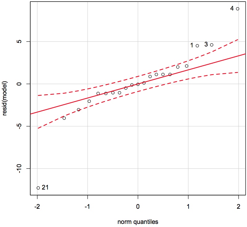
qqPlot(resid(model), id.method = "identify")
# Now use the mouse to click on the outliers and ID them # Right-click to stop adding points
From clicking on the points we see that observations 1, 3, 4 and 21 are quite unusual. </rst>
<rst> <rst-options: 'toc' = False/> <rst-options: 'reset-figures' = False/> These observations have residuals larger than what would be expected from a normal distribution. We don't exclude them yet. Let's examine if they appear in some of the other plots.
Leverage
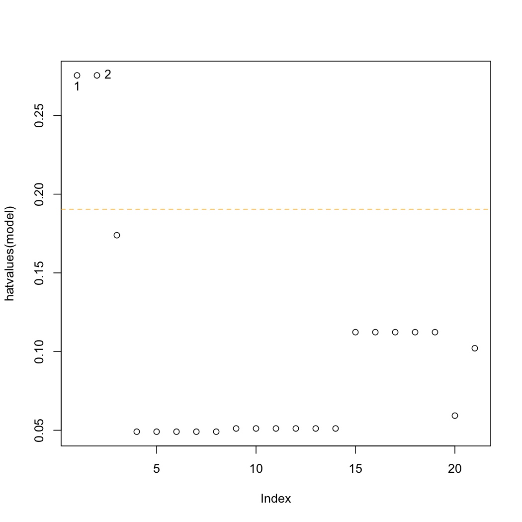
This is a plot of the hat-values:
.. code-block:: s
plot(hatvalues(model)) K <- length(coef(model)) N <- nrow(stackloss) hat.avg <- K/N abline(h=c(2,3)*hat.avg, lty=2, col=c("orange", "red")) identify(hatvalues(model))
The average hat value is at :math:`\overline{h} = k/n`. Observations 1 and 2 lie beyond only the 2 times the average hat value. We are more concerned with points that have hat values beyond 3 times the average. </rst>
<rst> <rst-options: 'toc' = False/> <rst-options: 'reset-figures' = False/> Discrepancy
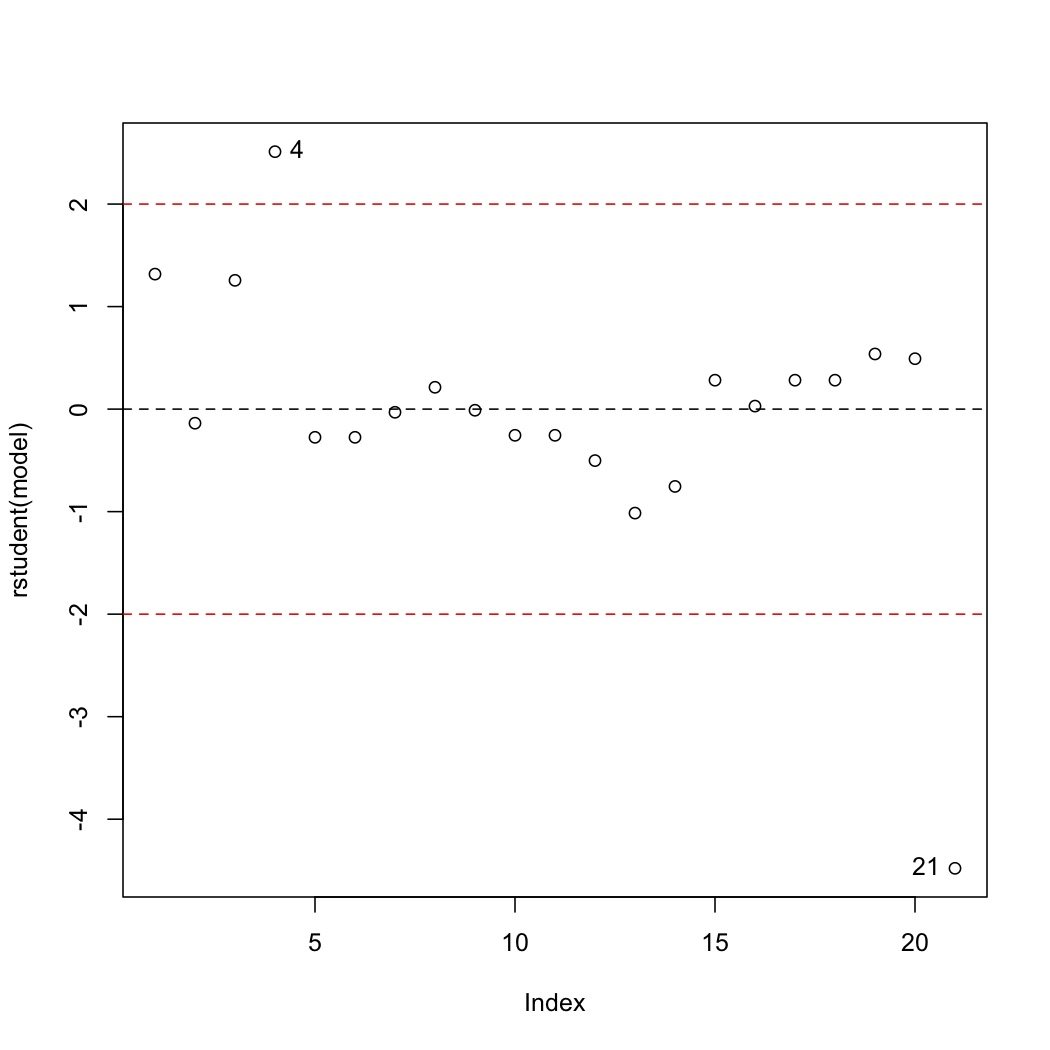
The discrepancy of each data point is found by plotting the studentized residuals:
.. code-block:: s
plot(rstudent(model)) abline(h=0, lty=2) abline(h=c(-2,2), lty=2, col="red") identify(rstudent(model))
Recall the cut-offs are at :math:`\pm 2` and contain 95% of the data (1 in 20 observations will naturally lie outside these limits). Observations 4 and 21 lie outside the limits and should be investigated. Specifically observation 4 is under-predicted (error = observed - predicted), while observation 21 is over-predicted.
Was there anything extra going on with those observations? Can another variable be included into the model that will reduce the size of the residuals for those points? </rst>
<rst> <rst-options: 'toc' = False/> <rst-options: 'reset-figures' = False/> Influence
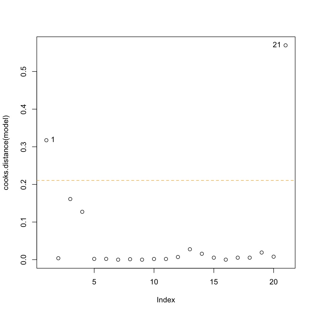
A plot of the Cook's D values shows influence. We loosely can describe influence as:
.. math::
\text{Influence} = \text{Leverage} \times \text{Discrepancy}
though Cook's D calculates leverage and discrepancy slightly differently from shown previously.
.. code-block:: s
plot(cooks.distance(model)) cutoff <- 4/model$df.residual abline(h=cutoff, lty=2, col=c("orange", "red")) identify(cooks.distance(model))
The cutoff for Cook's D is :math:`4/(n-k)`. Observations 1 and 21 lie beyond only the cutoff in this data set. Why did observation 1 show up, but not observation 2 (*answer*: both originally had high leverage, but observation 1 has higher residual error than observation 2). </rst>
<rst> <rst-options: 'toc' = False/> <rst-options: 'reset-figures' = False/> Combine leverage, discrepancy and influence to understand outliers
.. code-block:: s
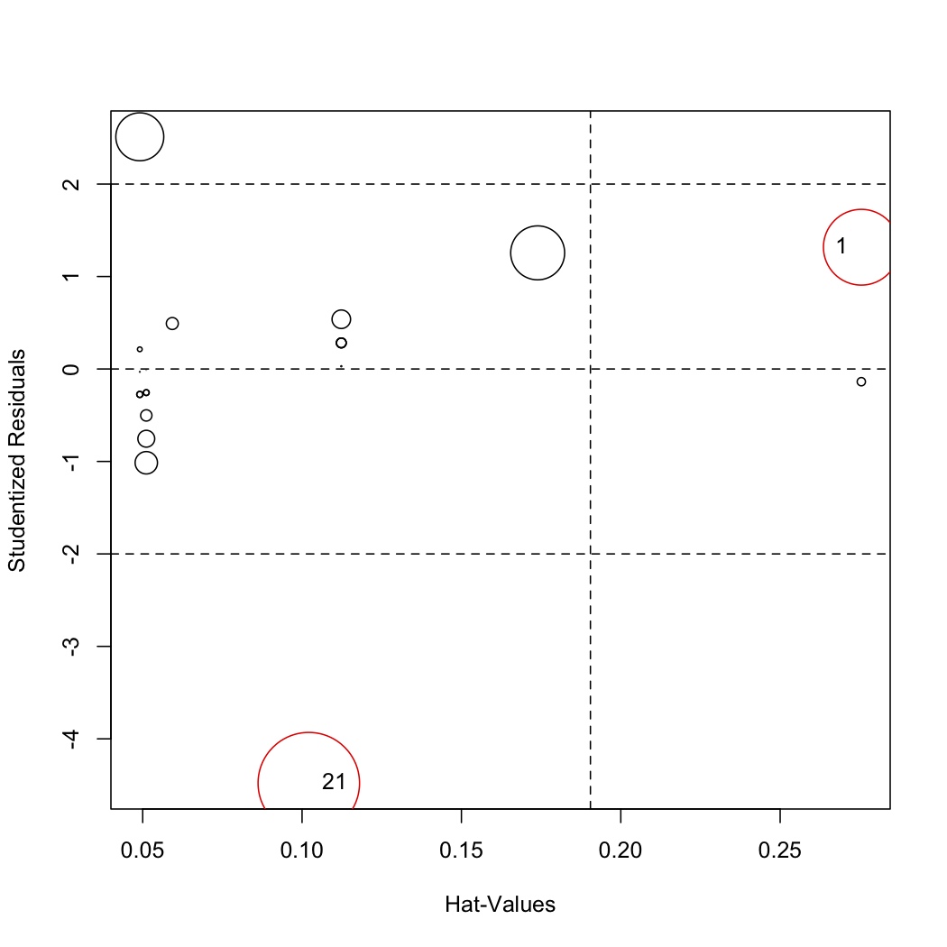
library(car) # Let the function auto-identify the outliers; tell it which labels to use influencePlot(model, id.method="noteworthy", labels=row.names(stackloss))
# Manually identify outliers with your mouse influencePlot(model, id.method="identify", labels=row.names(stackloss))
The auto-identify function marks only observations with large Cook's distance values. You should still investigate the other points. </rst>
<rst> <rst-options: 'toc' = False/> <rst-options: 'reset-figures' = False/> Also see ``influence(model)`` and ``influence.measures(model)`` for other metrics used to assess influence on a model from each observation.
Also, the ``influenceIndexPlot(model)`` function from the ``car`` library shows 4 different metrics of influence in 4 subplots and is useful for smallish data sets.
Removing outliers and rebuilding the model
After investigation of the points, we may decide to remove point 1 and 21 and rebuild the model:
.. code-block:: s
remove = -c(1, 21) model.rebuild <- lm(model, subset=remove)
Note how easy it is rebuild the model: you give it the existing ``model`` and the observations to remove (note the "``-``" in front of the ``c()``).
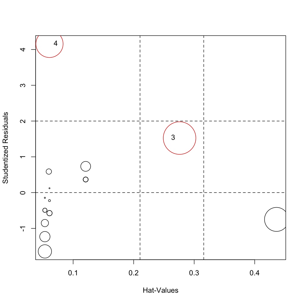
Then re-investigate the influence plot:
.. code-block:: s
influencePlot(model.rebuild, labels=row.names(stackloss)[remove]) </rst>
