Difference between revisions of "Software tutorial/Least squares modelling (linear regression)"
m |
|||
| Line 96: | Line 96: | ||
to show additional regression statistics. However, all the outputs from a linear model that we require for this course are computed in the code shown above. Python does not have a similar function (to my knowledge). | to show additional regression statistics. However, all the outputs from a linear model that we require for this course are computed in the code shown above. Python does not have a similar function (to my knowledge). | ||
= Regression when the intercept is zero = | |||
The above code can also be used in the case when | |||
= Multiple linear regression = | = Multiple linear regression = | ||
Revision as of 18:56, 2 December 2010
One of the best packages for fitting least squares models, in addition to all sorts of other statistical manipulation of data is the R language. The following pages from the 4C3 (Statistics for Engineering) website will help you:
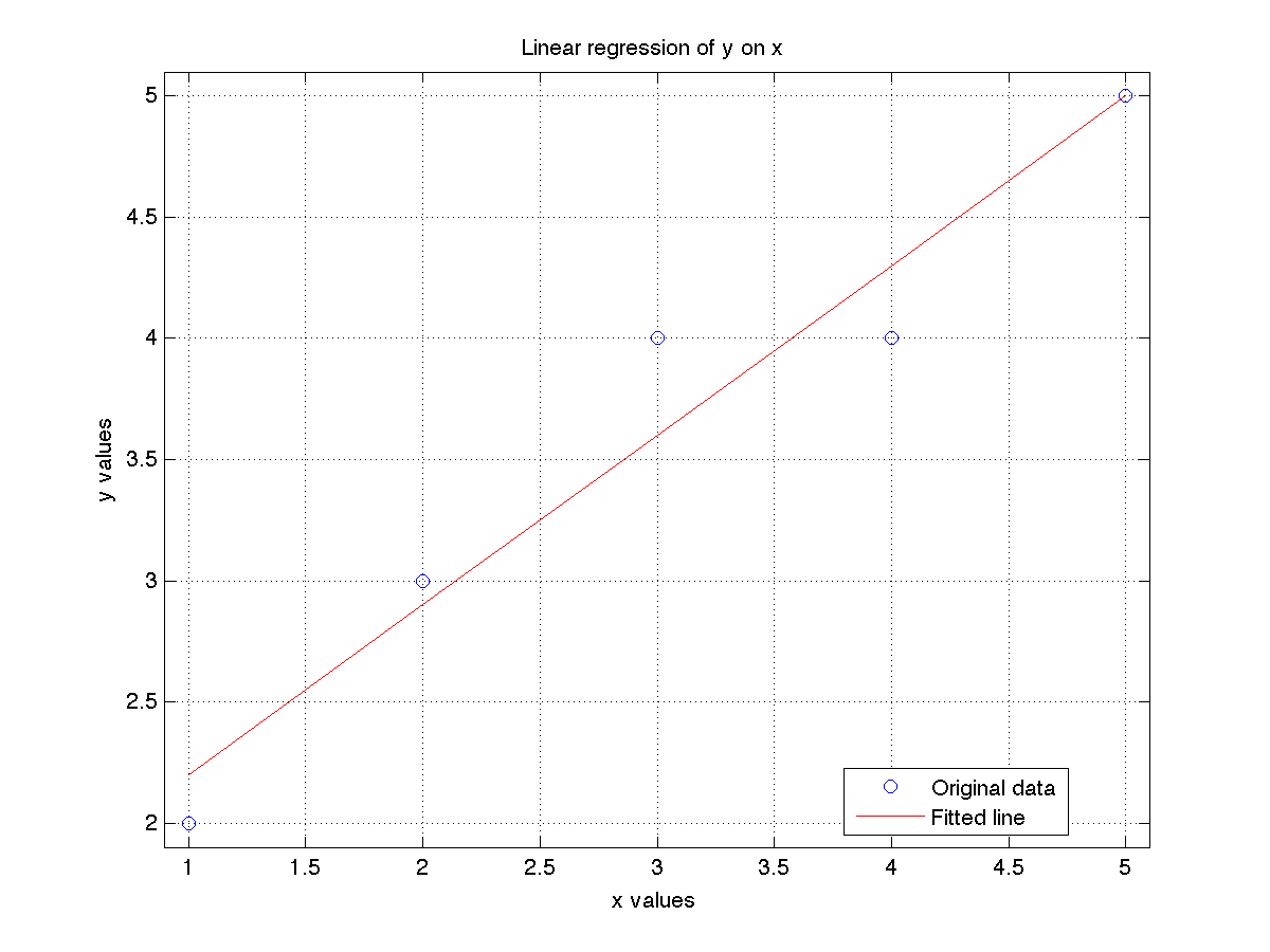
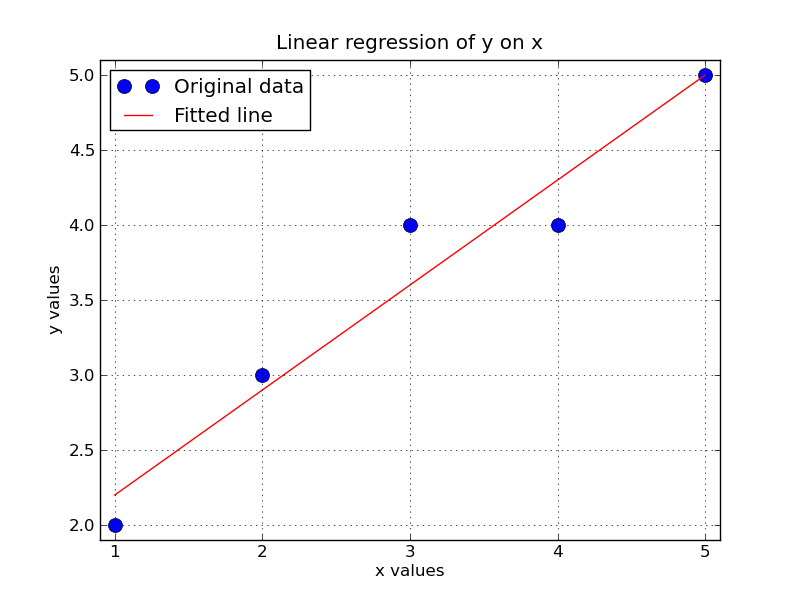
However, here is a tutorial on how you can use MATLAB or Python to fit a least squares model.
- MATLAB: use the regress.m and regstats.m function
- Python: use the numpy.linalg.lstsq function
Single-variable regression
| MATLAB | Python |
|---|---|
x = [1, 2, 3, 4, 5];
y = [2, 3, 4, 4, 5];
y = y(:);
n = numel(x);

X = [ones(n,1) x(:)];
a = regress(y, X)      % Contains a_0=a(1) and a_1=a(2)

% Plot the data along with the fitted line:
plot(x, y, 'o')
hold('on')
grid('on')
plot(x, X*a, 'r')
xlabel('x values')
ylabel('y values')
title('Linear regression of y on x')
xlim([0.9, 5.1])
ylim([1.9, 5.1])
legend({'Original data', 'Fitted line'}, 'Location', 'Best')

% Additional calculations
resids = y - X*a;            % resids = e = y - Xa
RSS = resids' * resids;      % residual sum of squares
TSS = sum((y - mean(y)).^2); % total sum of squares
R2 = 1 - RSS/TSS;

std_error = sqrt(RSS/(n-numel(a)));
std_y = sqrt(TSS/(n-1));     % just the same as std(y)
R2_adj = 1 - (std_error/std_y)^2
|
import numpy as np
from matplotlib.pyplot import *

x = np.array([1, 2, 3, 4, 5])
y = np.array([2, 3, 4, 4, 5])
n = len(x)

X = np.vstack([np.ones(n), x]).T
a = np.linalg.lstsq(X, y)[0]

# Plot the data along with the fitted line:
plot(x, y, 'o', label='Original data', markersize=10)
plot(x, np.dot(X,a), 'r', label='Fitted line')
xlabel('x values')
ylabel('y values')
title('Linear regression of y on x')
grid('on')
xlim([0.9, 5.1])
ylim([1.9, 5.1])
legend(loc=0)

# Additional calculations
resids = y - np.dot(X,a)       # e = y - Xa;
RSS = sum(resids**2)           # residual sum of squares
TSS = sum((y - np.mean(y))**2) # total sum of squares
R2 = 1 - RSS/TSS

std_error = np.sqrt(RSS/(n-len(a)))
std_y = np.sqrt(TSS/(n-1))   # just the same as std(y)
R2_adj = 1 - (std_error/std_y)**2
|
Matlab provides the function regstats that can be used as follows:
>> regstats(y, x)
to show additional regression statistics. However, all the outputs from a linear model that we require for this course are computed in the code shown above. Python does not have a similar function (to my knowledge).
Regression when the intercept is zero
The above code can also be used in the case when
Multiple linear regression
The case for multiple linear regression is identical to that shown above. The only difference is that you have to expand the X matrix with extra columns. The least squares coefficients in vector a are returned in the same order as the columns in matrix X.

