Software for integrating ODEs

Example

Consider the pair of differential equations (covered in a class on 11 February): <rst> <rst-options: 'toc' = False/> <rst-options: 'reset-figures' = False/> .. math::

\dfrac{dX}{dW} &= \dfrac{-r_A'}{F_{A0}} \\ \dfrac{dy}{dW} &= -\dfrac{\alpha}{2y}\left(1 + \varepsilon X\right)

Some terminology (recap from your pre-requisite math courses)

* The independent variable is \(W\) * The two dependent variables (variables being integrated with respect to the independent variable) are \(X\) and \(y\)

Since there are two dependent variables, we require initial conditions for each variable. In this case:

* :math:`X(0) = 0.0` * :math:`y(0) = 1.0`

We also need to specify initial **and final conditions** for the independent variable:

* :math:`W` initially is 0.0 at the reactor entrance * :math:`W` finally is 28.0 kg at the reactor exit

But there are a few other unknowns we must first specify:

* :math:`r_A' = -k' \dfrac{(1-X)y}{(1+\varepsilon*X)}` * :math:`q = \dfrac{(1 + \varepsilon X)}{y}` * :math:`F_{A0} = 0.1362\,\text{mol.s}^{-1}` * :math:`k' = 0.0074\,\text{mol.s}^{-1}\text{.(kg catalyst)}^{-1}` * :math:`\alpha = 0.0367\,\text{kg}^{-1}` * :math:`\varepsilon = -0.15` </rst>

Polymath

Download and install Polymath from the CD/DVD included with your course textbook (Windows only; sorry Mac and Linux versions are not available). Unfortunately this is only a 15 day version, which is pretty useless for this course, since you will require the code for at least the next 30 to 45 days. So rather use one of the other options below, if possible.

Enter the following Polymath code (as demonstrated in class on 11 February. Check the video out for a detailed explanation of the code.

# Differential equations
d(X) / d(W) = -rAdash / FA0 
X(0) = 0
d(y) / d(W) = -alpha/(2*y) * (1+eps*X) 
y(0) = 1.0

# Constants
FA0   = 0.1362  # [mol/s]
kdash = 0.0074  # [mol/(kg catalyst . s)]
alpha = 0.0367  # [1/kg]
eps   = -0.15   # [-]

# Algebraic equations
rAdash = -kdash * (1-X)/(1+eps*X) * y
flow_ratio = (1 + eps*X)/y

# Initial and final values for independent variable:
W(0) = 0
W(f) = 28

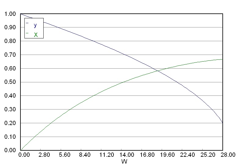
Ensure that you obtain a graphical output as shown here. This represents the profile of conversion, \(X\) and the pressure drop ratio \(y\) throughout the reactor.

Python

Installing Python

Installation differs from Windows to Linux to Mac. One Python distribution that works well for many people is the Enthought Python Distribution (EPD). Another one, especially for Windows users is Python(x,y).

Libraries required

You are ready to go if you enter the following without getting error messages:

import numpy as np
from scipy import integrate
from matplotlib.pylab import (plot, grid, xlabel, ylabel)

If you experience problems importing these libraries, then re-install your Python distribution using one of the two options listed above.

Source code

import numpy as np
from scipy import integrate
from matplotlib.pylab import *
 
def PBR_model(indep, depnt):
    """
    Dynamic balance for the packed bed reactor (PBR); demo problem class 05C

    indep: the independent ODE variable, such as time or length
    depnt: a vector of dependent variables

    X = depnt[0] = the conversion
    y = depnt[1] = the pressure ratio = P/P_0 = y

    Returns d(depnt)/d(indep) = a vector of ODEs
    """

    # Assign some variables for convenience of notation
    X = depnt[0]
    y = depnt[1]

    # Constants
    FA0   = 0.1362  # [mol/s]
    kdash = 0.0074  # [mol/(kg catalyst . s)]
    alpha = 0.0367  # [1/kg]
    eps   = -0.15   # [-]

    #Algebraic equations
    rAdash = -kdash * (1-X)/(1+eps*X) * y
    flow_ratio = (1 + eps*X)/y

    # Output from this ODE function must be a COLUMN vector, with n rows
    n = len(depnt) 
    d_depnt__d_indep = np.zeros((n,1))
    d_depnt__d_indep[0] = -rAdash / FA0 
    d_depnt__d_indep[1] = -alpha/(2*y) * (1+eps*X) 
    return d_depnt__d_indep
 
# The "driver" that will integrate the ODE(s):
# -----------
# Start by specifying the integrator:
# use ``vode`` with "backward differentiation formula"
r = integrate.ode(PBR_model).set_integrator('vode', method='bdf')

# Set the time range
indep_start = 0.0   # kg
indep_final = 28.0  # kg
delta = 1.0         # the results will be shown only at these ``delta`` points 
num_steps = np.floor((indep_final - indep_start)/delta) + 1 # Number of time steps: 1 extra for initial condition

# Set initial condition(s): for integrating variable and time!
X_indep_zero = 0.0   # i.e. X(W=0) = 0.0
y_indep_zero = 1.0   # i.e. y(W=0) = 1.0
r.set_initial_value([X_indep_zero, y_indep_zero], indep_start)

# Create vectors to store trajectories
W = np.zeros((num_steps, 1))
X = np.zeros((num_steps, 1))
y = np.zeros((num_steps, 1))
W[0] = indep_start
X[0] = X_indep_zero
y[0] = y_indep_zero

# Integrate the ODE(s) across each delta timestep
k = 1
while r.successful() and k < num_steps:
    r.integrate(r.t + delta)

    # Store the results to plot later
    W[k] = r.t
    X[k] = r.y[0]
    y[k] = r.y[1]
    k += 1

# All done!  Plot the trajectories:
plot(W, X)
grid('on')
xlabel('Catalyst weight, W [kg]')
ylabel('Conversion')

plot(W, y)
grid('on')
xlabel('Catalyst weight, W [kg]')
ylabel('Pressure drop ratio, y [-]')
show()

Ensure that you obtain a graphical output as shown here. This represents the profile of conversion, \(X\) and the pressure drop ratio \(y\) throughout the reactor.