Difference between revisions of "Software tutorial/Dealing with distributions"
Kevin Dunn (talk | contribs) (Created page with "{{Navigation|Book=Software tutorial|previous=Calculating statistics from a data sample|current=Tutorial index|next=Extending R with packages}} __NOTOC__ Values from various di...") |
Kevin Dunn (talk | contribs) |
||
| (One intermediate revision by the same user not shown) | |||
| Line 7: | Line 7: | ||
To calculate the probability value directly from *any* distribution in R you use a function created by combining ``d`` with the name of the distribution, that is what is meant by ``dDIST`` in the illustration here: | To calculate the probability value directly from *any* distribution in R you use a function created by combining ``d`` with the name of the distribution, that is what is meant by ``dDIST`` in the illustration here: | ||
[[Image:show-dDIST.jpg|500px|center]] | [[Image:show-dDIST.jpg|500px|center]] | ||
<rst> | <rst> | ||
| Line 80: | Line 80: | ||
* For the chi-squared distribution: ``rchisq(...)`` | * For the chi-squared distribution: ``rchisq(...)`` | ||
</rst> | </rst> | ||
{{Navigation|Book=Software tutorial|previous=Calculating statistics from a data sample|current=Tutorial index|next=Extending R with packages}} | |||
Latest revision as of 09:42, 13 January 2016
Values from various distribution functions are easily calculated in R.
Direct probability from a distribution
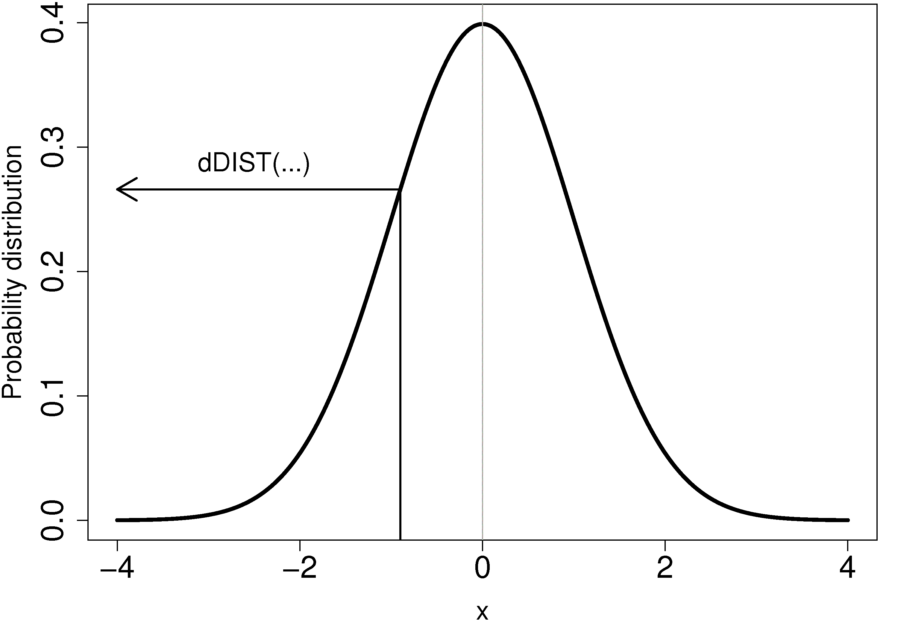
To calculate the probability value directly from *any* distribution in R you use a function created by combining ``d`` with the name of the distribution, that is what is meant by ``dDIST`` in the illustration here:
<rst> <rst-options: 'toc' = False/> <rst-options: 'reset-figures' = False/> For the *normal* distribution: ``dnorm(x=...)``
For example, ``dnorm(1)`` returns 0.2419707, the point of inflection on the normal distribution curve.
For the :math:`t` distribution: ``dt(x=..., df=...)`` where ``df`` are the degrees of freedom in the :math:`t`-distribution
For the :math:`F`-distribution: ``df(x=..., df1=..., df2=...)`` given the ``df1`` (numerator) and ``df2`` (denominator) degrees of freedom.
For the chi-squared distribution: ``dchisq(x=..., df=...)`` given the ``df`` degrees of freedom.
Values from the cumulative and inverse cumulative distribution
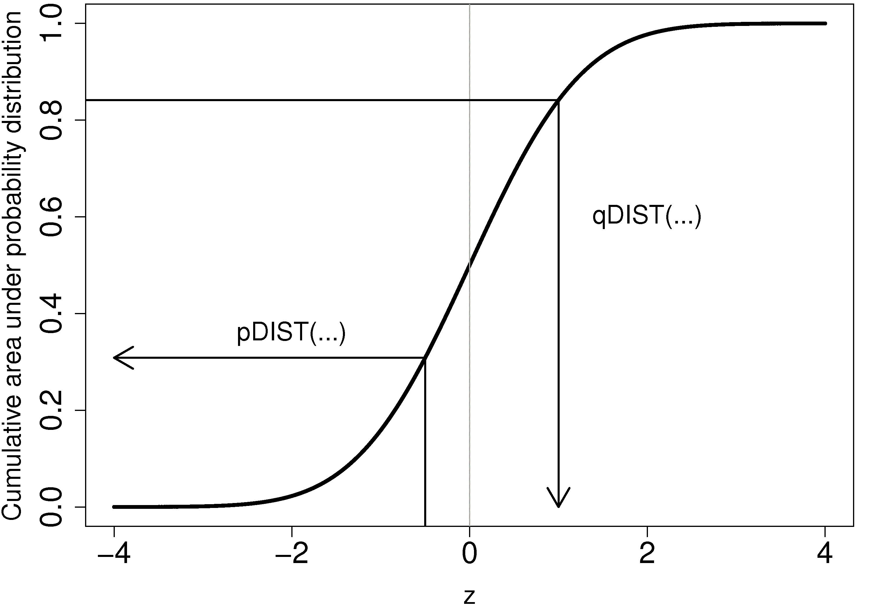
Similar to the above, we call the function by combining ``p`` - to get the cumulative percentage area under the distribution, and ``q`` - to get the quantile. </rst>
<rst> <rst-options: 'toc' = False/> <rst-options: 'reset-figures' = False/>
- For the *normal* distribution: ``pnorm(...)`` and ``qnorm(...)``
- For the :math:`t`-distribution: ``pt(...)`` and ``qt(...)``
- For the :math:`F`-distribution: ``pf(...)`` and ``qf(...)``
- For the chi-squared distribution: ``pchisq(...)`` and ``qchisq(...)``
Obtaining random numbers from a particular distribution
To obtain a single random number from the normal distribution with mean of 0 and standard deviation of 1.0:
.. code-block:: s
rnorm(1) [1] -0.3451397
For example, to obtain 10 random, normally distributed values:
.. code-block:: s
rnorm(10) [1] 0.4604076 -0.9670948 -0.2624246 -0.2223866 0.2492692 [6] 0.7160273 -0.2734768 2.4437870 0.4269511 -0.4831478
where the ``r`` prefix indicates we want random numbers.
Notice that R has used a default value of ``mean=0`` and *standard deviation* ``sd=1``. If you'd like your random numbers centred about a different mean, with a different level of spread, then:
.. code-block:: s
rnorm(n=10, mean=30, sd=4) [1] 31.62686 37.83101 28.07470 20.95000 30.47500 [6] 28.21797 35.81518 28.61481 30.59083 32.94051
Please pay attention to the fact that this function accepts the *standard deviation* and not the variance. In the previous example, the usual notation in statistics is to say :math:`x \sim \mathcal{N}(30, 16)` that is, we specify the variance, but the random number generator requires you specify the standard deviation.
- For the :math:`t` distribution: ``rt(...)``
- For the :math:`F`-distribution: ``rf(...)``
- For the chi-squared distribution: ``rchisq(...)``
</rst>

