Software for integrating ODEs
Background
Numerically integrating ODE's is something you should have mastered in your pre-requisite 3E4 course. If you are not familiar with this topic, it is your responsibility to quickly catch up, because we will use this intensively for the rest of the course.
Here is a tutorial a wrote a few years ago when I taught 3E4 in 2010. The tutorial below is similar, but uses a reactor design example.
Example
The example we will work with is a common modelling reaction: a liquid-based stirred tank reactor, with (initially) constant physical properties, a second order chemical reaction where species A is converted to B according to \({\sf A} \rightarrow {\sf B} \), with reaction rate \(r = k C_{\sf A}^2\). One can find the time-dependent mass balance for this system to be:
\[ \frac{dC_{\sf A}(t)}{dt} = \frac{F(t)}{V} \bigg( C_{{\sf A},\text{in}} - C_{\sf A} \bigg) - k C_{\sf A}^2 \]
where \(C_{{\sf A},\text{in}} = 5.5\) mol/L, we will initially assume constant volume of \(V = 100\) L and constant inlet flow of \(F(t) = 20.1 \) L/min. The reaction rate constant is 0.15 \(\frac{\text{L}}{\text{mol}.\text{min}}\). We must specify an initial condition for every differential equation: we will let \( C_{\sf A}(t=0) = 0.5\) mol/L.
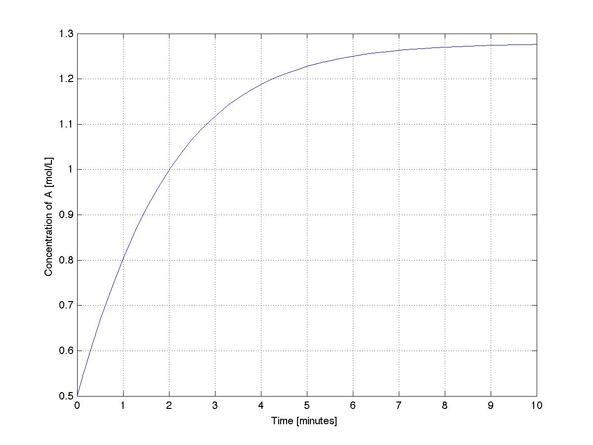
In the code below we will integrate the ODE from \(t_\text{start} = 0.0\) minutes up to \(t_\text{final} = 10.0\) minutes and plot the time-varying trajectory of concentration in the tank.
MATLAB code
In a file called tank.m:
function dydt = tank(t, y)

% Dynamic balance for a CSTR
%
% C_A = y(1) = the concentration of A in the tank, mol/L
%
% Returns dy/dt = F/V*(C_{A,in} - C_A) - k*C_A^2

F = 20.1;      % L/min
CA_in = 2.5;   % mol/L
V = 100;       % L
k = 0.150;     % L/(min.mol)

% Assign some variables for convenience of notation
CA = y(1);

% The output from the ODE function must be a COLUMN vector,
% with n rows
n = numel(y);       % How many ODE's in this system?
dydt = zeros(n,1);
dydt(1) = F/V*(CA_in - CA) - k*CA^2;
In a separate file (any name), for example: ode_driver.m, which will "drive" the ODE solver:
% Integrate the ODE
% -----------------

% Set the time range:
t_start = 0;
t_final = 10.0;

% Set the initial condition(s):
CA_t_zero = 0.5;

% Integrate the ODE(s):
[t, y] = ode45(@tank, [t_start, t_final], [CA_t_zero]);

% Plot the results:
clf;
plot(t, y)
grid('on')
xlabel('Time [minutes]')
ylabel('Concentration of A [mol/L]')
A plot from this code shows the system stabilizing after about 9 minutes.

Let's take a look at the MATLAB output:
>> t(1:10)
ans =
         0
    0.0689
    0.1378
    0.2067
    0.2757
    0.5257
    0.7757
    1.0257
    1.2757
    1.5257

>> y(1:10)
ans =
    0.5000
    0.5248
    0.5490
    0.5726
    0.5956
    0.6742
    0.7452
    0.8090
    0.8662
    0.9171
MATLAB places the points at unequal step sizes of time. This is what their documentation has to say:
- The MATLAB ODE solvers utilize these methods by taking a step, estimating the error at this step, checking to see if the value is greater than or less than the tolerance, and altering the step size accordingly. These integration methods do not lend themselves to a fixed step size. Using an algorithm that uses a fixed step size is dangerous since you can miss points where your signal frequency is greater than the solver frequency. Using a variable step ensures that a large step size is used for low frequencies and a small step size is used for high frequencies. The ODE solvers within MATLAB are optimized for a variable step, run faster with a variable step size, and clearly the results are more accurate.