Principal Component Analysis
Class 2 (16 September)
<pdfreflow> class_date = 16 September 2011 [1.65 Mb] button_label = Create my projector slides! show_page_layout = 1 show_frame_option = 1 pdf_file = lvm-class-2.pdf </pdfreflow> or you may download the lecture slides directly.
- Download these 3 CSV files and bring them on your computer:
- Peas dataset: http://datasets.connectmv.com/info/peas
- Food texture dataset: http://datasets.connectmv.com/info/food-texture
- Food consumption dataset: http://datasets.connectmv.com/info/food-consumption
Background reading
- Reading for class 2
- Linear algebra topics you should be familiar with before class 2:
- matrix multiplication
- that matrix multiplication of a vector by a matrix is a transformation from one coordinate system to another (we will review this in class)
- linear combinations (read the first section of that website: we will review this in class)
- the dot product of 2 vectors, and that they are related by the cosine of the angle between them (see the geometric interpretation section)
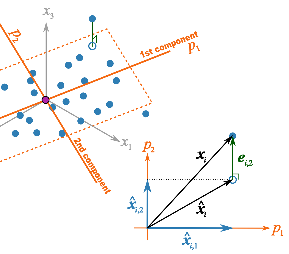
This illustration should help better explain what I trying to get across in class 2B
Class 3 (23 September)
I would advise printing the slides out no more than 2 per page (leaving space for extra notes in today's class) <pdfreflow> class_date = 23 September 2011 [580 Kb] button_label = Create my projector slides! show_page_layout = 1 show_frame_option = 1 pdf_file = lvm-class-3.pdf </pdfreflow> or you may download the lecture slides directly.
Background reading
- Least squares:
- what is the objective function of least squares
- how to calculate the regression coefficient
- understand that the residuals in least squares are orthogonal to
- Some optimization theory:
- How an optimization problem is written with equality constraints
- The Lagrange multiplier principle for solving simple, equality constrained optimization problems.
Class 4 (30 September)
Notes are the Process monitoring section.
Background reading
- Reading on cross validation
