Principal Component Analysis
Jump to navigation
Jump to search
The printable version is no longer supported and may have rendering errors. Please update your browser bookmarks and please use the default browser print function instead.
| Class date(s): | 16, 23, 30 September 2011 | ||||
| |||||
| |||||
| |||||
| |||||
| |||||
| |||||
| |||||
| |||||
Class 2 (16 September 2011)
![]() Download the class slides (PDF)
Download the class slides (PDF)
- Download these 3 CSV files and bring them on your computer:
- Peas dataset: http://openmv.net/info/peas
- Food texture dataset: http://openmv.net/info/food-texture
- Food consumption dataset: http://openmv.net/info/food-consumption
Background reading
- Reading for class 2
- Linear algebra topics you should be familiar with before class 2:
- matrix multiplication
- that matrix multiplication of a vector by a matrix is a transformation from one coordinate system to another (we will review this in class)
- linear combinations (read the first section of that website: we will review this in class)
- the dot product of 2 vectors, and that they are related by the cosine of the angle between them (see the geometric interpretation section)
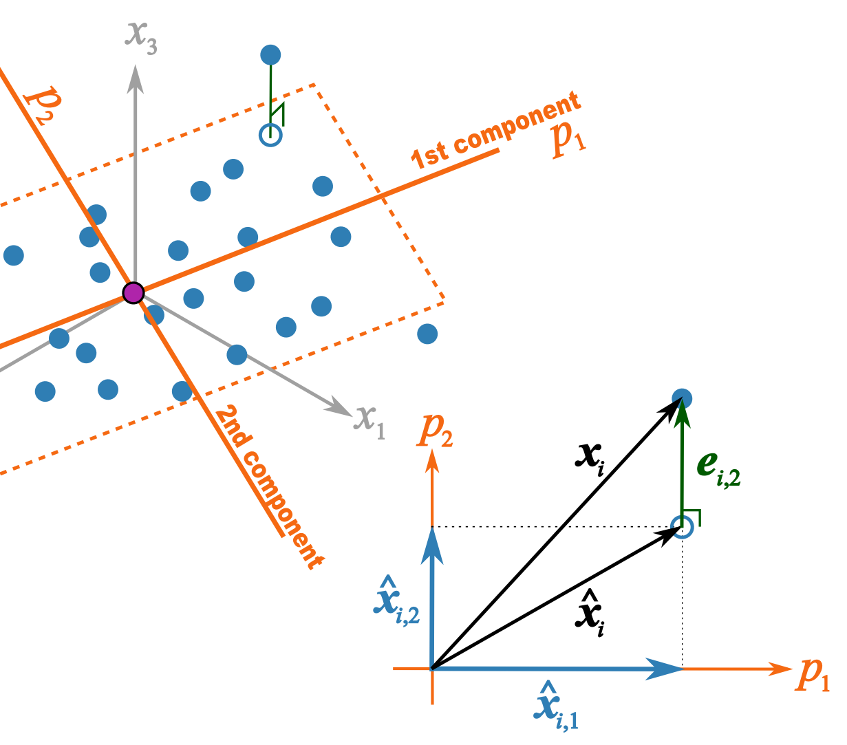
This illustration should help better explain what I trying to get across in class 2B
- \(p_1\) and \(p_2\) are the unit vectors for components 1 and 2.
- \( \mathbf{x}_i \) is a row of data from matrix \( \mathbf{X}\).
- \(\hat{\mathbf{x}}_{i,1} = t_{i,1}p_1\) = the best prediction of \( \mathbf{x}_i \) using only the first component.
- \(\hat{\mathbf{x}}_{i,2} = t_{i,2}p_2\) = the improvement we add after the first component to better predict \( \mathbf{x}_i \).
- \(\hat{\mathbf{x}}_{i} = \hat{\mathbf{x}}_{i,1} + \hat{\mathbf{x}}_{i,2} \) = is the total prediction of \( \mathbf{x}_i \) using 2 components and is the open blue point lying on the plane defined by \(p_1\) and \(p_2\). Notice that this is just the vector summation of \( \hat{\mathbf{x}}_{i,1}\) and \( \hat{\mathbf{x}}_{i,2}\).
- \(\mathbf{e}_{i,2} \) = is the prediction error vector because the prediction \(\hat{\mathbf{x}}_{i} \) is not exact: the data point \( \mathbf{x}_i \) lies above the plane defined by \(p_1\) and \(p_2\). This \(e_{i,2} \) is the residual distance after using 2 components.
- \( \mathbf{x}_i = \hat{\mathbf{x}}_{i} + \mathbf{e}_{i,2} \) is also a vector summation and shows how \( \mathbf{x}_i \) is broken down into two parts: \(\hat{\mathbf{x}}_{i} \) is a vector on the plane, while \( \mathbf{e}_{i,2} \) is the vector perpendicular to the plane.
Class 3 (23, 30 September 2011)
![]() Download the class slides (PDF)
Download the class slides (PDF)
Background reading
- Least squares:
- what is the objective function of least squares
- how to calculate the regression coefficient \(b\) for \(y = bx + e\) where \(x\) and \(y\) are centered vectors
- understand that the residuals in least squares are orthogonal to \(x\)
- Some optimization theory:
- How an optimization problem is written with equality constraints
- The Lagrange multiplier principle for solving simple, equality constrained optimization problems.
Background reading
- Reading on cross validation
