Isothermal reactor design - 2013
| Class date(s): | 04 February to 27 February | ||||
| |||||
| |||||
| |||||
| |||||
| |||||
| |||||
| |||||
- F2011: Chapter 5 and 6
- F2006: Chapter 4
04 February 2013 (05A)
- General problem solving strategy for reactor engineering
- Audio and video recording of the class
06 February 2013 (05B)
- The Ergun equation derivation
- Audio and video recording of the class
07 February 2013 (05C)
- Notes used during the class
- The spreadsheet with the Ergun equation example. Use it to try
- different lengths of reactor
- different catalyst particle sizes
- different pipe diameters
- gas properties (e.g. density)
- to see the effect on pressure drop in the packed bed.
11 February 2013 (06A)
- Audio and video recording of the class
- Codes to solve the example in class are available on the page software for integrating ODEs.
14 February 2013 (06C): midterm review
25 February 2013 (07A)
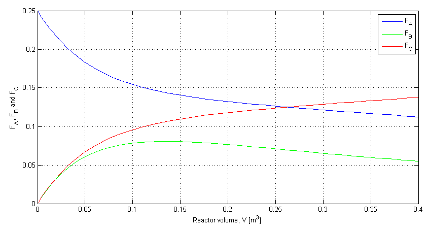
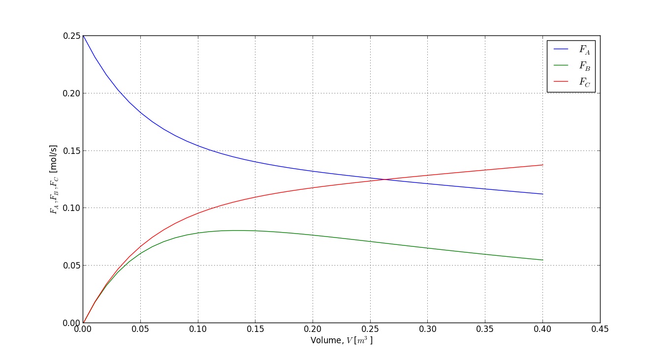
The example covered in class is based on example 4-8 in F2006 and example 6-2 in F2011. <rst> <rst-options: 'toc' = False/> <rst-options: 'reset-figures' = False/> The 3 ODE's are:
.. math::
\dfrac{dF_A}{dV} &= r_A\ \dfrac{dF_B}{dV} &= r_B - R_B \ \dfrac{dF_C}{dV} &= r_C
where :math:`-r_A = r_B = r_C` and :math:`-r_A = k\left(C_A - \dfrac{C_B C_C}{K_C} \right)`, and :math:`R_B = k_\text{diff}C_B`.
- :math:`k = 0.01\,\text{s}^{-1}`
- :math:`k_\text{diff} = 0.005\,\text{s}^{-1}`
- :math:`K_C = 50\,\text{mol.m}^{-3}`
We derived earlier in the course that
.. math:: C_A = C_\text{TO}\left(\dfrac{F_A}{F_T}\right)\left(\dfrac{P}{P_0}\right)\left(\dfrac{T_0}{T}\right)
Assuming isothermal and isobaric conditions in the membrane:
.. math:: C_A = C_\text{T0}\left(\dfrac{F_A}{F_T}\right)
where :math:`F_T = F_A + F_B + F_C` and :math:`C_\text{T0} = \dfrac{P_0}{RT_0}`. Similar equations can be written for :math:`C_B` and :math:`C_C`.
Using all of the above derivations, we can set up our numerical integration as shown below. </rst>
MATLAB
In a file called membrane.m:
function d_depnt__d_indep = membranem(indep, depnt)

% Dynamic balance for the packed bed reactor (PBR); demo problem class 05C
%
%    indep: the independent ODE variable, such as time or length
%    depnt: a vector of dependent variables
%
%    X = depnt(1) = the conversion
%    y = depnt(2) = the pressure ratio = P/P_0 = y
%
%    Returns d(depnt)/d(indep) = a vector of ODEs

% Assign some variables for convenience of notation
FA = depnt(1);
FB = depnt(2);
FC = depnt(3);

% Constants
kDiff = 0.005;  % s^{-1}
k = 0.01;       % s^{-1}
KC = 50;        % mol.m^{-3}
P0 = 830600;    % Pa
T0 = 500;       % K
R  = 8.314;     % J/(mol.K)

% Algebraic equations
FT = FA + FB + FC;
CT0 = P0 / (R * T0);
CA = CT0 * FA / FT;
CB = CT0 * FB / FT;
CC = CT0 * FC / FT;
RB = kDiff * CB;
rA = -k * (CA - CB * CC / KC);
rB = -rA;
rC = -rA;

% Output from this ODE function must be a COLUMN vector, with n rows
n = numel(depnt);
d_depnt__d_indep = zeros(n,1);
d_depnt__d_indep(1) = rA;
d_depnt__d_indep(2) = rB - RB;
d_depnt__d_indep(3) = rC;
In a separate file (any name), for example: ode_driver.m, which will "drive" the ODE solver:
% Integrate the ODE
% -----------------

% The independent variable always requires an initial and final value:
indep_start = 0.0;  % m^3
indep_final = 0.4;  % m^3

% Set initial condition(s): for integrating variables (dependent variables)
FA_depnt_zero = 0.25;   % i.e. FA(V=0) = 15 mol/min = 0.25 mol/s
FB_depnt_zero = 0.0;    % i.e. FB(V=0) = 0 mol/s
FC_depnt_zero = 0.0;    % i.e. FC(V=0) = 0 mol/s

% Integrate the ODE(s):
[V, depnt] = ode45(@membranem, [indep_start, indep_final], [FA_depnt_zero, FB_depnt_zero, FC_depnt_zero]);

% Plot the results:
clf;
plot(V, depnt(:,1), 'b')
grid('on')
hold('on')
plot(V, depnt(:,2), 'g')
plot(V, depnt(:,3), 'r')
xlabel('Reactor volume, V [m^3]')
ylabel('F_A, F_B and F_C')
legend('F_A', 'F_B', 'F_C')
Python
import numpy as np
from scipy import integrate
from matplotlib.pylab import (plot, grid, xlabel, ylabel, show, legend)

def membrane(indep, depnt):
    """
    Dynamic balance for the membrane reactor; class 07A

    indep: the independent ODE variable, such as time or length
    depnt: a vector of dependent variables

    X = depnt[0] = the conversion
    y = depnt[1] = the pressure ratio = P/P_0 = y

    Returns d(depnt)/d(indep) = a vector of ODEs
    """

    # Assign some variables for convenience of notation
    FA = depnt[0]
    FB = depnt[1]
    FC = depnt[2]

    # Constants
    kDiff = 0.005  # s^{-1}
    k = 0.01       # s^{-1}
    KC = 50        # mol.m^{-3}
    P0 = 830600    # Pa
    T0 = 500       # K
    R  = 8.314     # J/(mol.K)

    # Algebraic equations
    FT = FA + FB + FC
    CT0 = P0 / (R * T0)
    CA = CT0 * FA / FT
    CB = CT0 * FB / FT
    CC = CT0 * FC / FT
    R_B = kDiff * CB
    rA = -k * (CA - CB * CC / KC)
    rB = -rA
    rC = -rA

    # Output from this ODE function must be a COLUMN vector, with n rows
    n = len(depnt)
    d_depnt__d_indep = np.zeros((n,1))
    d_depnt__d_indep[0] = rA
    d_depnt__d_indep[1] = rB - R_B
    d_depnt__d_indep[2] = rC
    return d_depnt__d_indep

# The "driver" that will integrate the ODE(s):
# -----------
# Start by specifying the integrator:
# use ``vode`` with "backward differentiation formula"
r = integrate.ode(membrane).set_integrator('vode', method='bdf')

# Set the independent variable's range
indep_start = 0.0  # m^3
indep_final = 0.4  # m^3
delta = 0.01       # the results will be shown only at these ``delta`` points
num_steps = np.floor((indep_final - indep_start)/delta) + 1 # Number of steps: 1 extra for initial condition

# Set initial condition(s): for integrating variables (dependent variables)
FA_depnt_zero = 0.25   # i.e. FA(V=0) = 15 mol/min = 0.25 mol/s
FB_depnt_zero = 0.0    # i.e. FB(V=0) = 0 mol/s
FC_depnt_zero = 0.0    # i.e. FC(V=0) = 0 mol/s

r.set_initial_value([FA_depnt_zero, FB_depnt_zero, FC_depnt_zero], indep_start)

# Create vectors to store trajectories
V = np.zeros((num_steps, 1))
FA = np.zeros((num_steps, 1))
FB = np.zeros((num_steps, 1))
FC = np.zeros((num_steps, 1))
V[0] = indep_start
FA[0] = FA_depnt_zero
FB[0] = FB_depnt_zero
FC[0] = FC_depnt_zero

# Integrate the ODE(s) across each delta
k = 1
while r.successful() and k < num_steps:
    r.integrate(r.t + delta)

    # Store the results to plot later
    V[k] = r.t
    FA[k] = r.y[0]
    FB[k] = r.y[1]
    FC[k] = r.y[2]
    k += 1

# All done!  Plot the trajectories:
plot(V, FA)
grid('on')
plot(V, FB)
plot(V, FC)
xlabel('Volume, $V$ [$m^3$]')
ylabel('$F_A, F_B, F_C$ [mol/s]')
legend(['$F_A$', '$F_B$', '$F_C$'])
show()
Polymath
d(FA)/d(V) = rA
d(FB)/d(V) = rB - RB
d(FC)/d(V) = rC

FA(0) = 0.25  # mol/s
FB(0) = 0.0   # mol/s
FC(0) = 0.0   # mol/s

# Independent variable
V(0) = 0
V(f) = 0.4  #m^3

# Constants
kDiff = 0.005  # s^{-1}
k = 0.01       # s^{-1}
KC = 50        # mol.m^{-3}
P0 = 830600    # Pa
T0 = 500       # K
R  = 8.314     # J/(mol.K)

# Algebraic equations
FT = FA + FB + FC
CT0 = P0 / (R * T0)
CA = CT0 * FA / FT
CB = CT0 * FB / FT
CC = CT0 * FC / FT
RB = kDiff * CB
rA = -k * (CA - CB * CC / KC)
rB = -rA
rC = -rA

