5.10. Blocking and confounding for disturbances
5.10.1. Characterization of disturbances
External disturbances will always have an effect on our response variable, \(y\). Operators, ambient conditions, physical equipment, lab analyses, and time-dependent effects (catalyst deactivation, fouling), will impact the response. This is why it is crucial to randomize the order of experiments: so that these unknown, unmeasurable, and uncontrollable disturbances cannot systematically affect the response.
However, certain disturbances are known, or controllable, or measurable. For these cases we perform pairing and blocking. We have already discussed pairing in the univariate section: pairing is when two experiments are run on the same subject and we analyze the differences in the two response values, rather than the actual response values. If the effect of the disturbance has the same magnitude on both experiments, then that disturbance will cancel out when calculating the difference. The magnitude of the disturbance is expected to be different between paired experiments, but is expected to be the same within the two values of the pair.
Blocking is slightly different: blocking is a special way of running the experiment so that the disturbance actually does affect the response, but we construct the experiment so that this effect is not misleading.
Finally, a disturbance can be characterized as a controlled disturbance, in which case it isn’t a disturbance anymore, as it is held constant for all experiments, and its effect cancels out. But it might be important to investigate the controlled disturbance, especially if the system is operated later on when this disturbance is at a different level.
5.10.2. Blocking and confounding
It is common for known, or controllable or measurable factors to have an effect on the response. However these disturbance factors might not be of interest to us during the experiment. Cases are:
Known and measurable, not controlled: Reactor vessel A is known to achieve a slightly better response, on average, than reactor B. However both reactors must be used to complete the experiments in the short time available.
Known, but not measurable nor controlled: There is not enough material to perform all \(2^3\) runs, there is only enough for 4 runs. The impurity in either the first batch A for 4 experiments, or the second batch B for the other 4 runs will be different, and might either increase or decrease the response variable (we don’t know the effect it will have).
Known, measurable and controlled: Reactor vessel A and B have a known, measurable effect on the output, \(y\). To control for this effect we perform all experiments in either reactor A or B, to prevent the reactor effect from confounding (confusing) our results.
In this section then we will deal with disturbances that are known, but their effect may or may not be measurable. We will also assume that we cannot control that disturbance, but we would like to minimize its effect.
For example, if we don’t have enough material for all \(2^3\) runs, but only enough for 4 runs, the question is how to arrange the 2 sets of 4 runs so that the known, by unmeasurable disturbance from the impurity has the least effect on our results and interpretation of the 3 factors.
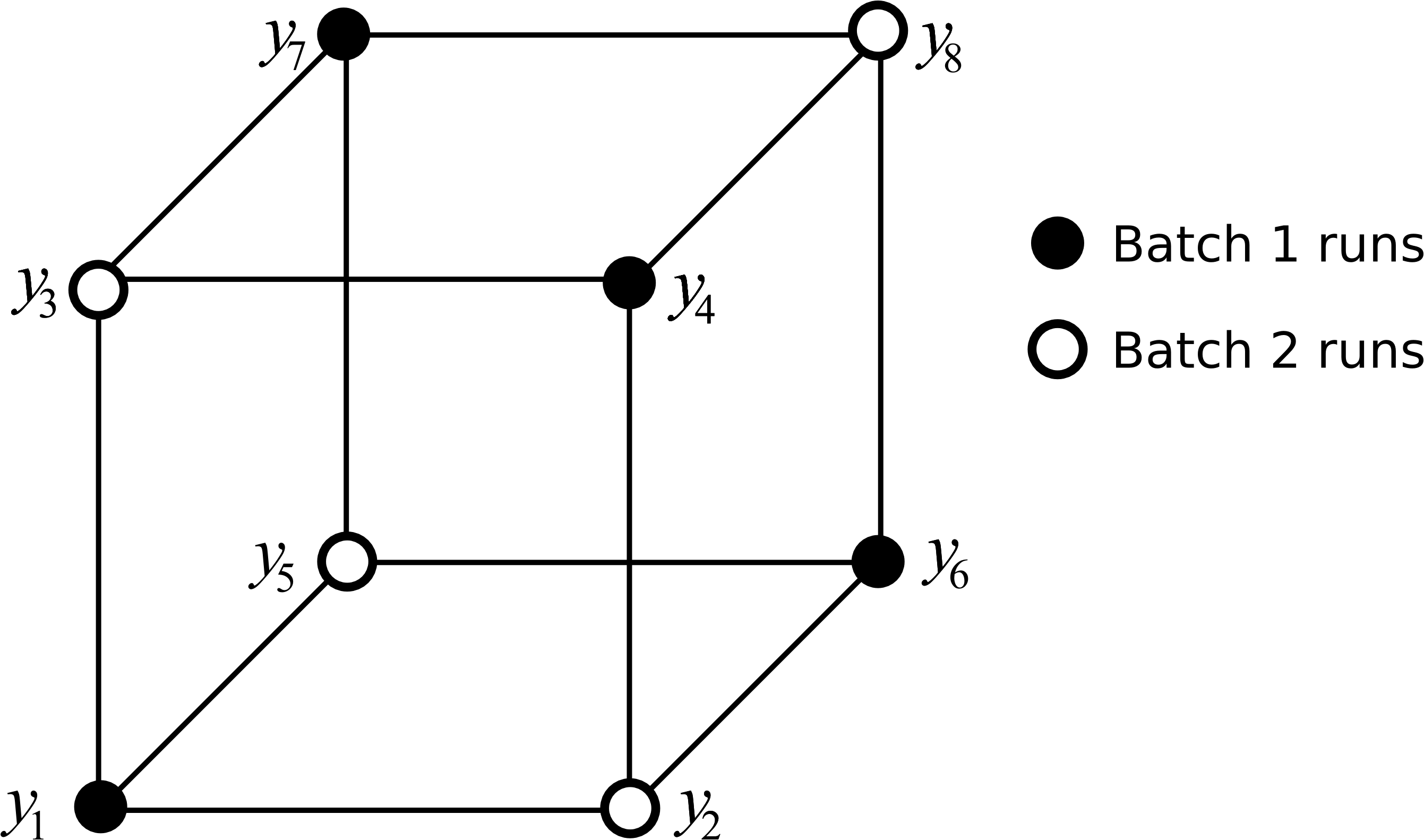
Our approach is to intentionally confound the effect of the disturbance with an effect that is expected to be the least significant. The \(A \times B \times C\) interaction term is almost always going to be small for many systems, so we will split the runs that the first 4 are run at the low level of \(ABC\) and the other four at the high level, as illustrated.
Each group of 4 runs is called a block and the process of creating these 2 blocks is called blocking. The experiments within each block must be run randomly.
Experiment |
A |
B |
C |
AB |
AC |
BC |
ABC |
Response, \(y\) |
|---|---|---|---|---|---|---|---|---|
1 |
\(-\) |
\(-\) |
\(-\) |
\(+\) |
\(+\) |
\(+\) |
\(-\) (batch 1) |
\(\widetilde{y}_1\) |
2 |
\(+\) |
\(-\) |
\(-\) |
\(-\) |
\(-\) |
\(+\) |
\(+\) (batch 2) |
\(\mathring{y}_2\) |
3 |
\(-\) |
\(+\) |
\(-\) |
\(-\) |
\(+\) |
\(-\) |
\(+\) (batch 2) |
\(\mathring{y}_3\) |
4 |
\(+\) |
\(+\) |
\(-\) |
\(+\) |
\(-\) |
\(-\) |
\(-\) (batch 1) |
\(\widetilde{y}_4\) |
5 |
\(-\) |
\(-\) |
\(+\) |
\(+\) |
\(-\) |
\(-\) |
\(+\) (batch 2) |
\(\mathring{y}_5\) |
6 |
\(+\) |
\(-\) |
\(+\) |
\(-\) |
\(+\) |
\(-\) |
\(-\) (batch 1) |
\(\widetilde{y}_6\) |
7 |
\(-\) |
\(+\) |
\(+\) |
\(-\) |
\(-\) |
\(+\) |
\(-\) (batch 1) |
\(\widetilde{y}_7\) |
8 |
\(+\) |
\(+\) |
\(+\) |
\(+\) |
\(+\) |
\(+\) |
\(+\) (batch 2) |
\(\mathring{y}_8\) |
If the raw material has a significant effect on the response variable, then we will not be able to tell whether it was due to the \(A \times B \times C\) interaction, or due to the raw material, since \(\hat{\beta}_{ABC} \rightarrow \underbrace{\text{ABC interaction}}_{\text{expected to be small}} + \text{raw material effect}\).
But the small loss due to this confusion of effects, is the gain that we can still estimate the main effects and two-factor interactions without bias, provided the effect of the disturbance is constant. Let’s see how we get this result by denoting \(\widetilde{y}_i\) as a \(y\) response from the first batch of materials and let \(\mathring{y}_i\) denote a response from the second batch.
Using the least squares equations you can show for yourself that (some are intentionally left blank for you to complete):
\[\begin{split}\hat{\beta}_A &= -\widetilde{y}_1 + \mathring{y}_2 - \mathring{y}_3 + \widetilde{y}_4 - \mathring{y}_5 + \widetilde{y}_6 - \widetilde{y}_7 + \mathring{y}_8 \\ \hat{\beta}_B &= \\ \hat{\beta}_C &= \\ \hat{\beta}_{AB} &= +\widetilde{y}_1 - \mathring{y}_2 - \mathring{y}_3 + \widetilde{y}_4 + \mathring{y}_5 - \widetilde{y}_6 - \widetilde{y}_7 + \mathring{y}_8\\ \hat{\beta}_{AC} &= \\ \hat{\beta}_{BC} &= \\ \hat{\beta}_{ABC} &= \\\end{split}\]
Imagine now the \(y\) response was increased by \(g\) units for the batch 1 experiments, and increased by \(h\) units for batch 2 experiments. You can prove to yourself that these biases will cancel out for all main effects and all two-factor interactions. The three factor interaction of \(\hat{\beta}_{ABC}\) will however be heavily confounded.
Another way to view this problem is that the first batch of materials and the second batch of materials can be represented by a new variable, called \(D\) with value of \(D_{-} =\) batch 1 and \(D_{+} =\) batch 2. We will show next that we must consider this new factor to be generated from the other three: D = ABC.
We will also address the case when there are more than two blocks in the next section on the use of generators. For example, what should we do if we have to run a \(2^3\) factorial but with only enough material for 2 experiments at a time?