5.9.8. Design foldover

Experiments are not a one-shot operation. They are almost always sequential, as we learn more and more about our system. Once the first screening experiments are complete there will always be additional questions. In this section we consider two common questions that arise after an initial set of fractional factorials have been run.

Dealias a single main effect (switch sign of one factor)

In the previous example we had a \(2^{7-4}_{\text{III}}\) system with generators D=AB, E=AC, F=BC, and G=ABC. Effect C was the largest effect. But we cannot be sure it was large due to factor C alone: it might have been one of the interactions it is aliased with. The aliasing pattern for effect C was: \(\widehat{\beta}_{\mathbf{C}} \rightarrow\) C + AE + BF + DG. For example, we might have reason to believe the AE interaction is large. We would like to do some additional experiments so that C becomes unconfounded with any two-factor interactions.

The way we can do this is to run another 8 experiments, but this time just change the sign of C to -C; in other words, re-run the original 8 experiments where the only thing that is changed is to flip the signs on column C; the columns which are generated from column C should remain as they were. This implies that the generators have become D=AB, E=-AC, F=-BC, and G=-ABC. We must emphasize, do not re-create these generated columns from new signs in column C. What we have now is another \(2^{7-4}_{\text{III}}\) design. You can calculate the aliasing pattern for the recent 8 experiments is \(\widehat{\beta}_{\mathbf{C}} \rightarrow\) C - AE - BF - DG.

Now consider putting all 16 runs together and analyzing the joint results. There are now 16 parameters that can be estimated. Using computer software you can see that factor C will have no confounding with any two-factor interactions. Also, any two-factor interactions involving C are removed from the other main effects. For example, factor A was originally confounded with CE with the first 8 experiments; but that will be removed when analyzing all 16 together.

So our general conclusion is: switching the sign of one factor will de-alias that factor’s main effect, and all its associated two-factor interactions when analyzing the two fractional factorials together. In the above example, we will have an unconfounded estimate of C and 2-factor interactions involving C will be unconfounded with main effects: i.e. AC, BC, CD, CE, CF and CG.

Increase design resolution (switching all signs)

One can improve the aliasing structure of a design when switching all the signs of all factors from the first fraction. Switching the signs means that we take the complete design matrix of factor settings, and simply flip the signs to create the second fraction. A factor setting that was run at the low level in the first fraction is then run at a high level in the second fraction. This includes generated factors: imagine that D = AB, and we had A \(=-1\), B \(=+1\) for a particular run in the first fraction. In the first fraction we would have D \(= (-1)(+1) = -1\), while in the second fraction it would simply be D \(=+1\), with A \(=+1\) and B \(=-1\) respectively, since we simply flip signs. We do not regenerate the generated factors.

In the \(2^{7-4}_\text{III}\) example, we ran 8 experiments. If we now run another 8 experiments with all the signs switched, then these 8+8 experiments would be equivalent to a \(2^{7-3}_\text{IV}\) design. This resolution IV design means that all the main effects can now be estimated without confounding from any two-factor interactions. However, the two-factor interactions are still confounded with themselves.

This is a good strategy in general: to run the first fraction of runs to assess the main effects. It serves as a good checkpoint, as well providing intermediate results to colleagues, it can be used to get approval/budget to run the next set of experiments. If we then perform another set of runs we know that we are doing them in a way that captures the most additional information, and with the least confounding. Remember experimentation is not done in a single go; it is sequential. We perform experiments, analyze the results, and design further experiments to reach our goal.

5.9.9. Projectivity

A final observation for this section is how fractional factorials will collapse down to a full factorial under certain conditions.

Consider the diagram here, where a half fraction in factors A, B and C was run (4 experiments) at the closed points.

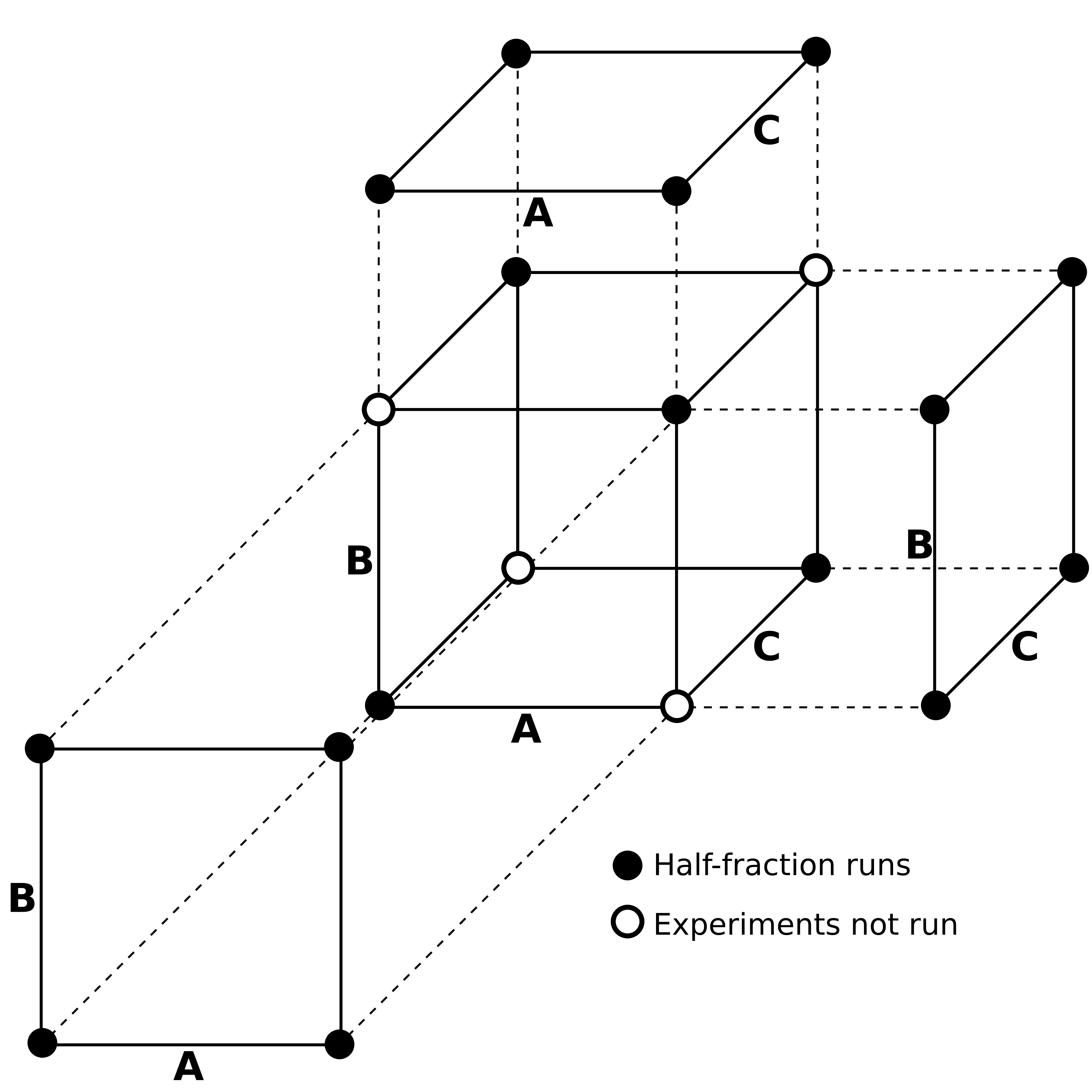
On analyzing the data, the experimenter discovers that factor C does not actually have an impact on response \(y\). This means the C dimension could have been removed from the experiment, and is illustrated by projecting the A and B factors forward, removing factor C. Notice that this is now a full factorial in factors A and B. The same situation would hold if either factor B or factor A were found to be unimportant. Furthermore if two factors are found to be unimportant, then this corresponds to 2 replicate experiments in 1 factor.

This projectivity of factorials holds in general for a larger number of factors. The above example, actually a \(2^{3-1}_\text{III}\) experiment, was a case of projectivity = 2. In general, projectivity = \(P\) = resolution \(-\) 1. So if you have a resolution IV fractional factorial, then it has projectivity = \(P = 4 - 1\), implying that it contains a full factorial in 3 factors. So a \(2^{6-2}_\text{IV}\) (16 runs) system with 6 factors, contains an embedded full factorial using a combination of any 3 factors; if any 3 factors were found unimportant, then a replicated full factorial exists in the remaining 3 factors.