2.10. Poisson distribution

The Poisson distribution is useful to characterize rare events (number of cell divisions in a small time unit), system failures and breakdowns, or number of flaws on a product (contaminations per cubic millimetre). These are events that have a very small probability of occurring within a given time interval or unit area (e.g. pump failure probability per minute = 0.000002), but there are many opportunities for the event to possibly occur (e.g. the pump runs continuously). A key assumption is that the events must be independent. If one pump breaks down, then the other pumps must not be affected; if one flaw is produced per unit area of the product, then other flaws that appear on the product must be independent of the first flaw.

Let \(n\) = number of opportunities for the event to occur. If this is a time-based system, then it would be the number of minutes the pump is running. If it were an area/volume based system, then it might be the number of square inches or cubic millimetres of the product. Let \(p\) = probability of the event occurring: e.g. \(p = 0.000002\) chance per minute of failure, or \(p = 0.002\) of a flaw being produced per square inch. The rate at which the event occurs is then given by \(\eta = np\) and is a count of events per unit time or per unit area. A value for \(p\) can be found using long-term, historical data.

There are two important properties:

1. The mean of the distribution for the rate happens to be the rate at which unusual events occur = \(\eta = np\)

2. The variance of the distribution is also \(\eta\). This property is particularly interesting - state in your own words what this implies.

Formally, the Poisson distribution can be written as \(\displaystyle \frac{e^{-\eta}\eta^{x}}{x!}\), with a plot as shown for \(\eta = 4\). Please note the lines are only guides, the probability is only defined at the integer values marked with a circle.

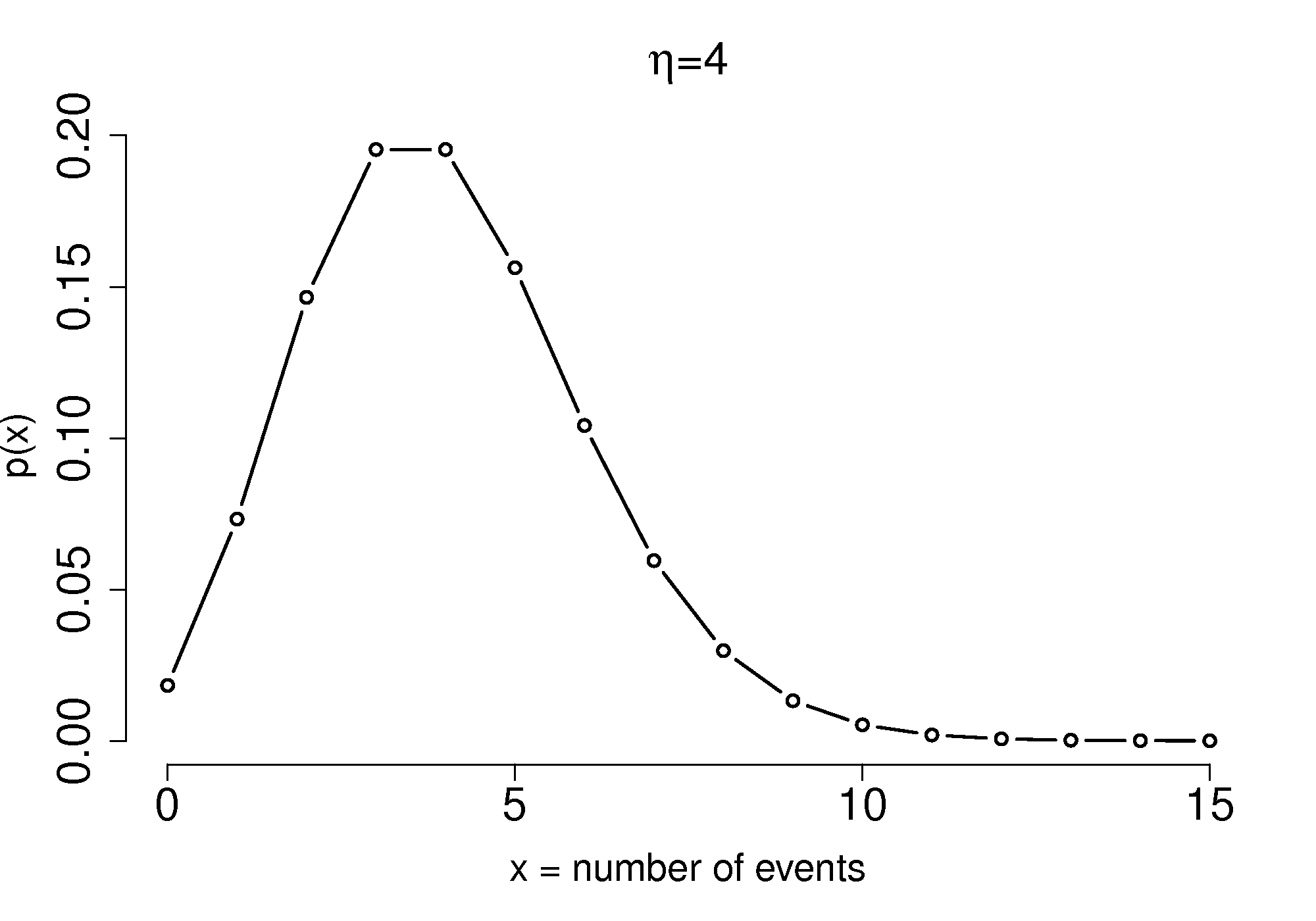
\(p(x)\) expresses the probability that there will be \(x\) occurrences (must be an integer) of this rare event in the same interval of time or unit area as \(\eta\) was measured.

Example: Equipment in a chemical plant can and will fail. Since it is a rare event, let’s use the Poisson distribution to model the failure rates. Historical records on a plant show that a particular supplier’s pumps are, on average, prone to failure in a month with probability \(p = 0.01\) (1 in 100 chance of failure each month). There are 50 such pumps in use throughout the plant. What is the probability that either 0, 1, 3, 6, 10, or 15 pumps will fail this year? (Create a table)

\(\eta = 12\,\frac{\displaystyle \text{months}}{\displaystyle \text{year}} \times 50\,\text{pumps} \times 0.01\,\frac{\displaystyle\text{failure}}{\displaystyle\text{month}} = 6\,\frac{\displaystyle\text{pump failures}}{\displaystyle\text{year}}\)

\(x\)	\(p(x)\)
0	0.25% chance
1	1.5%
3	8.9
6	16%
10	4.1%
15	0.1%