6.6. Principal Component Regression (PCR)
Principal component regression (PCR) is an alternative to multiple linear regression (MLR) and has many advantages over MLR.
In multiple linear regression we have two matrices (blocks): \(\mathbf{X}\), an \(N \times K\) matrix whose columns we relate to the single vector, \(\mathbf{y}\), an \(N \times 1\) vector, using a model of the form: \(\mathbf{y} = \mathbf{Xb}\). The solution vector \(\mathbf{b}\) is found by solving \(\mathbf{b} = \left(\mathbf{X'X}\right)^{-1}\mathbf{X'y}\). The variance of the estimated solution is given by \(\mathcal{V}(\mathbf{b}) = \left(\mathbf{X'X}\right)^{-1}S_E^2\).
In the section on factorial experiments we intentionally set our process to generate a matrix \(\mathbf{X}\) that has independent columns. This means that each column is orthogonal to the others, you cannot express one column in terms of the other, and it results in a diagonal \(\mathbf{X'X}\) matrix.
On most data sets though the columns in \(\mathbf{X}\) are correlated. Correlated columns are not too serious if they are mildly correlated. But the illustration here shows the problem with strongly correlated variables, in this example \(x_1\) and \(x_2\) are strongly, positively correlated. Both variables are used to create a predictive model for \(y\). The model plane, \(\hat{y}=b_0 + b_1x_1 + b_2x_2\) is found so that it minimizes the residual error. There is a unique minimum for the sum of squares of the residual error (i.e. the objective function). But very small changes in the raw \(x\)-data lead to almost no change in the objective function, but will show large fluctuations in the solution for \(\mathbf{b}\) as the plane rotates around the axis of correlation. This can be visualized in this illustration.
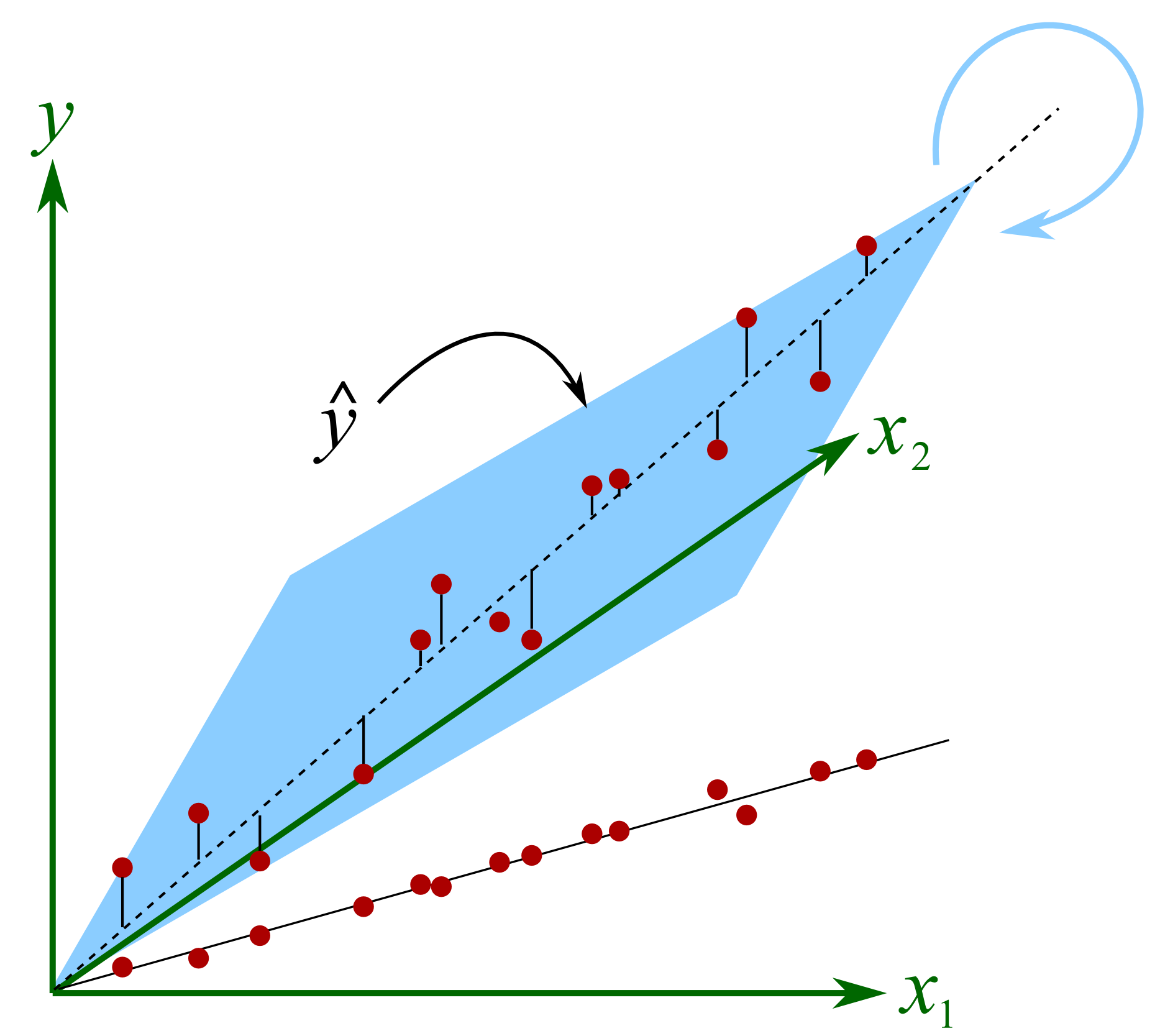
The plane will rotate around the axial, dashed line if we make small changes in the raw data. At each new rotation we will get very different values of \(b_1\) and \(b_2\), even changing in sign(!), but the objective function’s minimum value does not change very much. This phenomena shows up in the least squares solution as wide confidence intervals for the coefficients, since the off-diagonal elements in \(\mathbf{X'X}\) will be large. This has important consequences when you are trying to learn about your process from this model: you have to use caution. A model with low or uncorrelated variables is well-supported by the data, and cannot be arbitrarily rotated.
The common “solution” to this problem of collinearity is to revert to variable selection. In the above example the modeller would select either \(x_1\) or \(x_2\). In general, the modeller must select a subset of uncorrelated columns from the \(K\) columns in \(\mathbf{X}\) rather than using the full matrix. When \(K\) is large, then this becomes a large computational burden. Further, it is not clear what the trade-offs are, and how many columns should be in the subset. When is a correlation too large to be problematic?
We face another problem with MLR: the assumption that the variables in \(\mathbf{X}\) are measured without error, which we know to be untrue in many practical engineering situations and is exactly what leads to the instability of the rotating plane. Furthermore, MLR cannot handle missing data. To summarize, the shortcomings of multiple linear regression are that:
it cannot handle strongly correlated columns in \(\mathbf{X}\)
it assumes \(\mathbf{X}\) is noise-free, which it almost never is in practice
cannot handle missing values in \(\mathbf{X}\)
MLR requires that \(N > K\), which can be impractical in many circumstances, which leads to
variable selection to meet the \(N > K\) requirement, and to gain independence between columns of \(\mathbf{X}\), but that selection process is non-obvious, and may lead to suboptimal predictions.
The main idea with principal component regression is to replace the \(K\) columns in \(\mathbf{X}\) with their uncorrelated \(A\) score vectors from PCA.
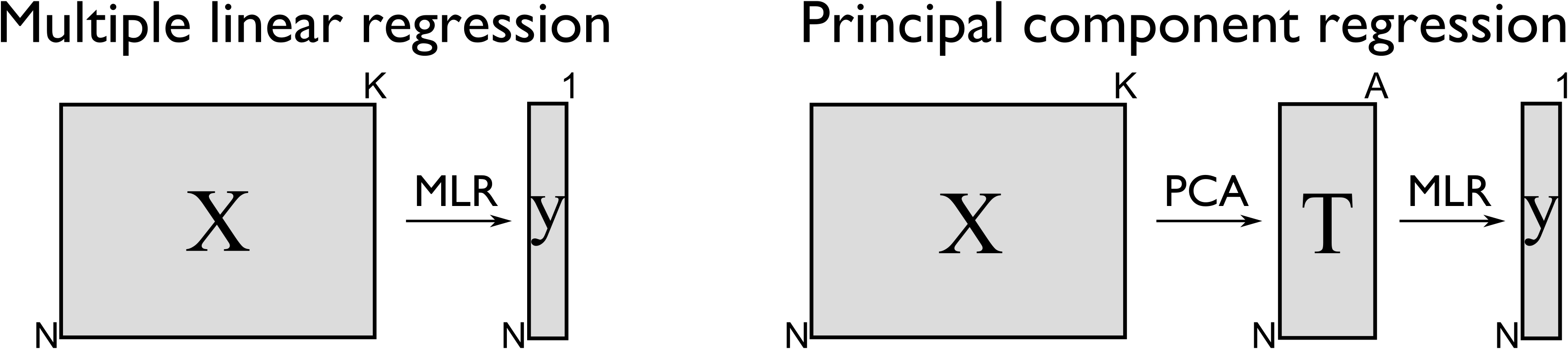
In other words, we replace the \(N \times K\) matrix of raw data with a smaller \(N \times A\) matrix of data that summarizes the original \(\mathbf{X}\) matrix. Then we relate these \(A\) scores to the \(\mathrm{y}\) variable. Mathematically it is a two-step process:
This has a number of advantages:
The columns in \(\mathbf{T}\), the scores from PCA, are orthogonal to each other, obtaining independence for the least-squares step.
These \(\mathbf{T}\) scores can be calculated even if there are missing data in \(\mathbf{X}\).
We have reduced the assumption of errors in \(\mathbf{X}\), since \(\widehat{\mathbf{X}} = \mathbf{TP' + E}\). We have replaced it with the assumption that there is no error in \(\mathbf{T}\), a more realistic assumption, since PCA separates the noise from the systematic variation in \(\mathbf{X}\). The \(\mathbf{T}\text{'s}\) are expected to have much less noise than the \(\mathbf{X}\text{'s}\).
The relationship of each score column in \(\mathbf{T}\) to vector \(\mathrm{y}\) can be interpreted independently of each other.
Using MLR requires that \(N > K\), but with PCR this changes to \(N > A\); an assumption that is more easily met for short and wide \(\mathbf{X}\) matrices with many correlated columns.
There is much less need to resort to selecting variables from \(\mathbf{X}\); the general approach is to use the entire \(\mathbf{X}\) matrix to fit the PCA model. We actually use the correlated columns in \(\mathbf{X}\) to stabilize the PCA solution, much in the same way that extra data improves the estimate of a mean (recall the central limit theorem).
But by far one of the greatest advantages of PCR though is the free consistency check that one gets on the raw data, which you don’t have for MLR. Always check the SPE and Hotelling’s \(T^2\) value for a new observation during the first step. If SPE is close to the model plane, and \(T^2\) is within the range of the previous \(T^2\) values, then the prediction from the second step should be reasonable.
Illustrated as follows we see the misleading strategy that is regularly seen with MLR. The modeller has build a least squares model relating \(x_1\) and \(x_2\) to \(y\), over the given ranges of \(x\). The closed circles represent the actual data, while the open circles are the projections of the \(x_1\) and \(x_2\) values on the \(x_1 - x_2\) plane. The predictive model works adequately.
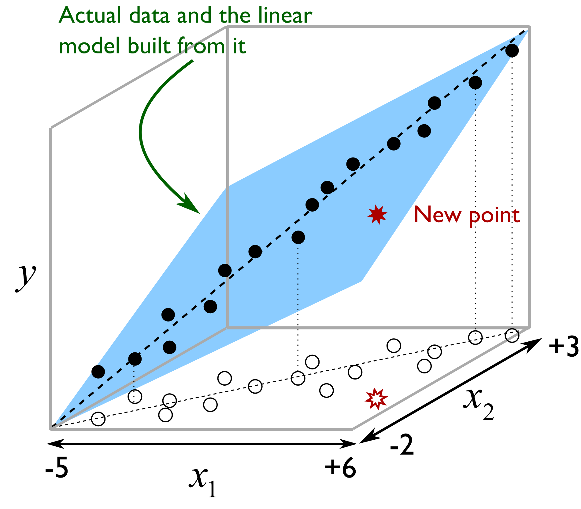
But the misleading strategy often used by engineers is to say that the model is valid as long as \(-5 \leq x_1 \leq +6\) and \(-2 \leq x_2 \leq +1\). If the engineer wants to use the model at the points marked with *, the results will be uncertain, even though those marked points obey the given constraints. The problem is that the engineer has not taken the correlation between the variables into account. With PCR we would immediately detect this: the points marked as * would have large SPE values from the PCA step, indicating they are not consistent with the model.
Here then is the procedure for building a principal component regression model.
Collect the \(\mathbf{X}\) and \(\mathrm{y}\) data required for the model.
Build a PCA model on the data in \(\mathbf{X}\), fitting \(A\) components. We usually set \(A\) by cross-validation, but often components beyond this will be useful. Iterate back to this point after the initial model to assess if \(A\) should be changed.
Examine the SPE and \(T^2\) plots from the PCA model to ensure the model is not biased by unusual outliers.
Use the columns in \(\mathbf{T}\) from PCA as your data source for the usual multiple linear regression model (i.e. they are now the \(\mathbf{X}\)-variables in an MLR model).
Solve for the MLR model parameters, \(\mathbf{b} = \left(\mathbf{T'T}\right)^{-1}\mathbf{T'y}\), an \(A \times 1\) vector, with each coefficient entry in \(\mathbf{b}\) corresponding to each score.
Using the principal component regression model for a new observation:
Obtain your vector of new data, \(\mathbf{x}'_\text{new, raw}\), a \(1 \times K\) vector.
Preprocess this vector in the same way that was done when building the PCA model (usually just mean centering and scaling) to obtain \(\mathbf{x}'_\text{new}\)
Calculate the scores for this new observation: \(\mathbf{t}'_\text{new} = \mathbf{x}'_{\text{new}} \mathbf{P}\).
Find the predicted value of this observation: \(\widehat{\mathbf{x}}'_\text{new} = \mathbf{t}'_\text{new} \mathbf{P}'\).
Calculate the residual vector: \(\mathbf{e}'_\text{new} = \mathbf{x}'_{\text{new}} - \widehat{\mathbf{x}}'_\text{new}\).
Then compute the residual distance from the model plane: \(\text{SPE}_\text{new} = \sqrt{\mathbf{e}'_\text{new} \mathbf{e}_\text{new}}\)
And the Hotelling’s \(T^2\) value for the new observation: \(T^2_\text{new} = \displaystyle \sum_{a=1}^{a=A}{\left(\dfrac{t_{\text{new},a}}{s_a}\right)^2}\).
Before calculating the prediction from the PCR model, first check if the \(\text{SPE}_\text{new}\) and \(T^2_\text{new}\) values are below their 95% or 99% limits. If the new observation is below these limits, then go on to calculate the prediction: \(\widehat{y}_\text{new} = \mathbf{t}'_\text{new}\mathbf{b}\), where \(\mathbf{b}\) was from the
If either of the \(\text{SPE}\) or \(T^2\) limits were exceeded, then one should investigate the contributions to SPE, \(T^2\) or the individuals scores to see why the new observation is unusual.
Predictions of \(\widehat{y}_\text{new}\) when a point is above either limit, especially the SPE limit, are not to be trusted.
Multiple linear regression, though relatively simpler to implement, has no such consistency check on the new observation’s \(x\)-values. It simply calculates a direct prediction for \(\widehat{y}_\text{new}\), no matter what the values are in \(\mathbf{x}_{\text{new}}\).
One of the main applications in engineering for PCR is in the use of software sensors, also called inferential sensors. The method of PLS has some distinct advantages over PCR, so we prefer to use that method instead, as described next.