6.5.16. Determining the number of components to use in the model with cross-validation
Cross-validation is a general tool that helps to avoid over-fitting - it can be applied to any model, not just latent variable models.
As we add successive components to a model we are increasing the size of the model, \(A\), and we are explaining the model-building data, \(\mathbf{X}\), better and better. (The equivalent in least squares models would be to add additional \(\mathbf{X}\)-variable terms to the model.) The model’s \(R^2\) value will increase with every component. As the following equation shows, the variance of the \(\widehat{\mathbf{X}}\) matrix increases with every component, while the residual variance in matrix \(\mathbf{E}\) must decrease.
This holds for any model where the \(\widehat{\mathbf{X}}\) and \(\mathbf{E}\) matrices are completely orthogonal to each other: \(\widehat{\mathbf{X}}'\mathbf{E} = \mathbf{0}\) (a matrix of zeros), such as in PCA, PLS and least squares models.
There comes a point for any real data set where the number of components, \(A\) = the number of columns in \(\mathbf{T}\) and \(\mathbf{P}\), extracts all systematic variance from \(\mathbf{X}\), leaving unstructured residual variance in \(\mathbf{E}\). Fitting any further components will start to fit this noise, and unstructured variance, in \(\mathbf{E}\).
Cross-validation for multivariate data sets was described by Svante Wold in his paper on Cross-validatory estimation of the number of components in factor and principal components models, in Technometrics, 20, 397-405, 1978.
The general idea is to divide the matrix \(\mathbf{X}\) into \(G\) groups of rows. These rows should be selected randomly, but are often selected in order: row 1 goes in group 1, row 2 goes in group 2, and so on. We can collect the rows belonging to the first group into a new matrix called \(\mathbf{X}_{(1)}\), and leave behind all the other rows from all other groups, which we will call group \(\mathbf{X}_{(-1)}\). So in general, for the \(g^\text{th}\) group, we can split matrix \(\mathbf{X}\) into \(\mathbf{X}_{(g)}\) and \(\mathbf{X}_{(-g)}\).
Wold’s cross-validation procedure asks to build the PCA model on the data in \(\mathbf{X}_{(-1)}\) using \(A\) components. Then use data in \(\mathbf{X}_{(1)}\) as new, testing data. In other words, we preprocess the \(\mathbf{X}_{(1)}\) rows, calculate their score values, \(\mathbf{T}_{(1)} = \mathbf{X}_{(1)} \mathbf{P}\), calculate their predicted values, \(\widehat{\mathbf{X}}_{(1)} = \mathbf{T}_{(1)} \mathbf{P'}\), and their residuals, \(\mathbf{E}_{(1)} = \mathbf{X}_{(1)} - \widehat{\mathbf{X}}_{(1)}\). We repeat this process, building the model on \(\mathbf{X}_{(-2)}\) and testing it with \(\mathbf{X}_{(2)}\), to eventually obtain \(\mathbf{E}_{(2)}\).
After repeating this on \(G\) groups, we gather up \(\mathbf{E}_{1}, \mathbf{E}_{2}, \ldots, \mathbf{E}_{G}\) and assemble a type of residual matrix, \(\mathbf{E}_{A,\text{CV}}\), where the \(A\) represents the number of components used in each of the \(G\) PCA models. The \(\text{CV}\) subscript indicates that this is not the usual error matrix, \(\mathbf{E}\). From this we can calculate a type of \(R^2\) value. We don’t call this \(R^2\), but it follows the same definition for an \(R^2\) value. We will call it \(Q^2_A\) instead, where \(A\) is the number of components used to fit the \(G\) models.
We also calculate the usual PCA model on all the rows of \(\mathbf{X}\) using \(A\) components, then calculate the usual residual matrix, \(\mathbf{E}_A\). This model’s \(R^2\) value is:
The \(Q^2_A\) behaves exactly as \(R^2\), but with two important differences. Like \(R^2\), it is a number less than 1.0 that indicates how well the testing data, in this case testing data that was generated by the cross-validation procedure, are explained by the model. The first difference is that \(Q^2_A\) is always less than the \(R^2\) value. The other difference is that \(Q^2_A\) will not keep increasing with each successive component, it will, after a certain number of components, start to decrease. This decrease in \(Q^2_A\) indicates the new component just added is not systematic: it is unable to explain the cross-validated testing data. We often see plots such as this one:
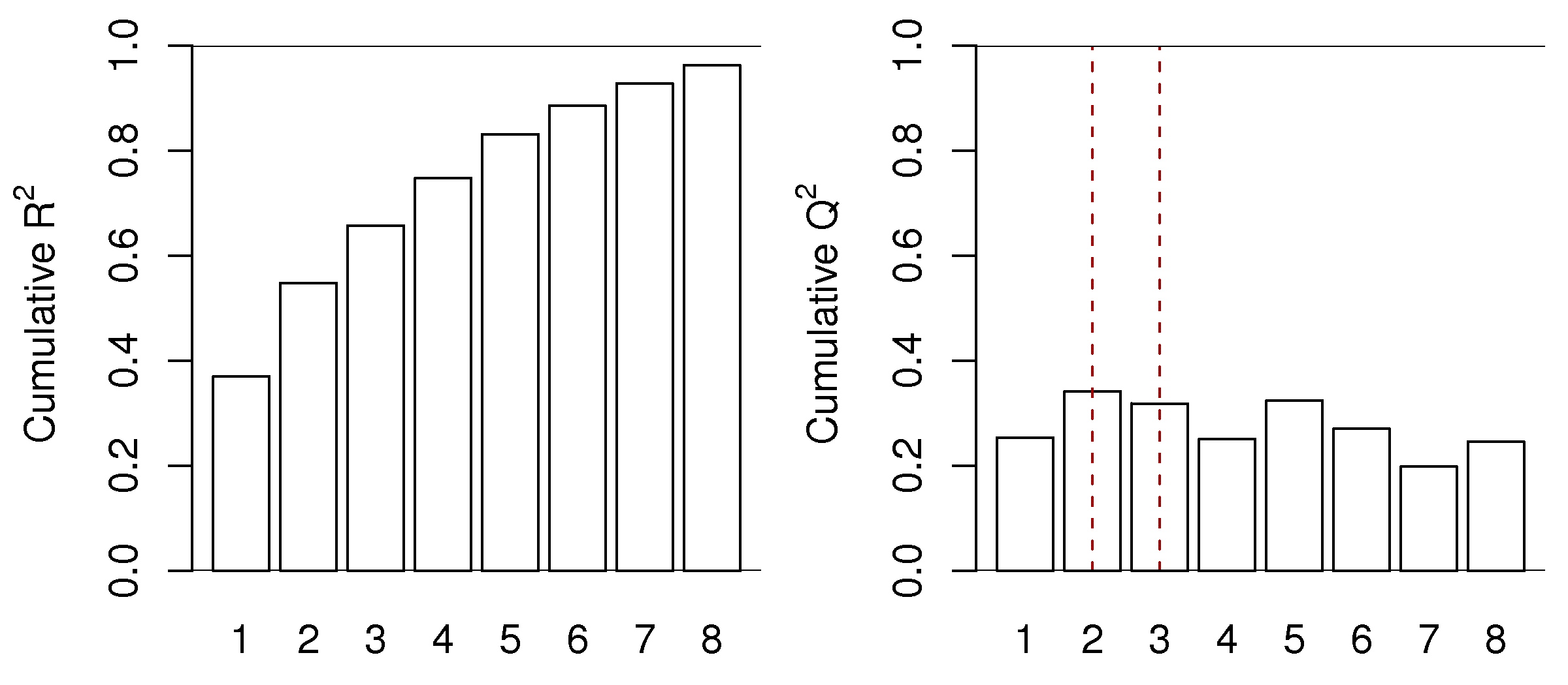
This is for a real data set, so the actual cut off for the number of components could be either \(A =2\) or \(A=3\), depending on what the 3rd component shows to the user and how interested they are in that component. Likely the 4th component, while boosting the \(R^2\) value from 66% to 75%, is not really fitting any systematic variation. The \(Q^2\) value drops from 32% to 25% when going from component 3 to 4. The fifth component shows \(Q^2\) increasing again. Whether this is fitting actual variability in the data or noise is for the modeller to determine, by investigating that 5th component. These plots show that for this data set we would use between 2 and 5 components, but not more.
Cross-validation, as this example shows is never a precise answer to the number of components that should be retained when trying to learn more about a dataset. Many studies try to find the “true” or “best” number of components. This is a fruitless exercise; each data set means something different to the modeller and the objective for which the model was intended to assist.
The number of components to use should be judged by the relevance of each component. Use cross-validation as guide, and always look at a few extra components and step back a few components; then make a judgement that is relevant to your intended use of the model.
However, cross-validation’s objective is useful for predictive models, such as PLS, so we avoid over-fitting components. Models where we intend to learn from, or optimize, or monitor a process may well benefit from fewer or more components than suggested by cross-validation.