6.5.17. Some properties of PCA models

We summarize various properties of the PCA model, most have been described in the previous sections. Some are only of theoretical interest, but others are more practical.

• The model is defined by the direction vectors, or loadings vectors, called \(\mathbf{p}_1, \mathbf{p}_2, \ldots, \mathbf{p}_A\); each are a \(K \times 1\) vector, and can be collected into a single matrix, \(\mathbf{P}\), a \(K \times A\) loadings matrix.

• These vectors form a line for one component, a plane for 2 components, and a hyperplane for 3 or more components. This line, plane or hyperplane define the latent variable model.

• An equivalent interpretation of the model plane is that these direction vectors are oriented in such a way that the scores have maximal variance for that component. No other directions of the loading vector (i.e. no other hyperplane) will give a greater variance.

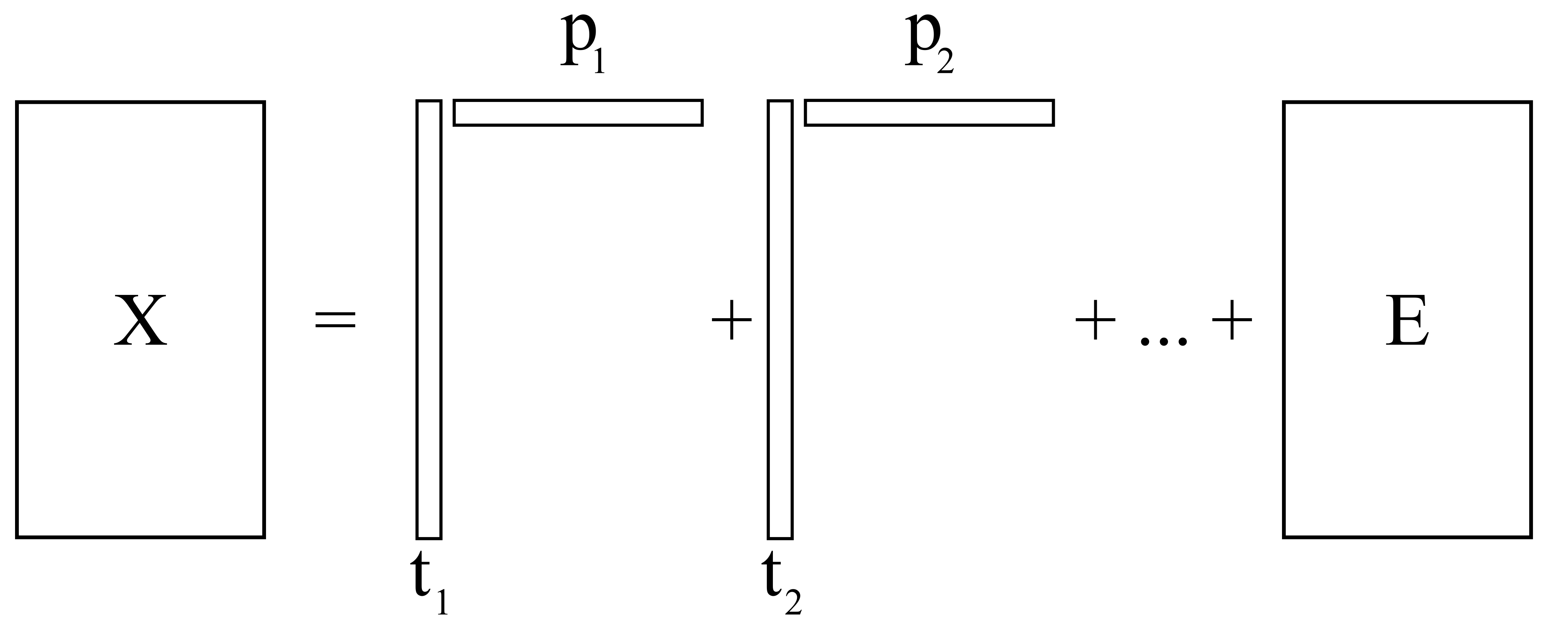
• This plane is calculated with respect to a given data set, \(\mathbf{X}\), an \(N \times K\) matrix, so that the direction vectors best-fit the data. We can say then that with one component, the best estimate of the original matrix \(\mathbf{X}\) is:

  \[\widehat{\mathbf{X}}_1 = \mathbf{t}_1 \mathbf{p}_1 \qquad \text{or equivalently:} \qquad \mathbf{X}_1 = \mathbf{t}_1 \mathbf{p}_1 + \mathbf{E}_1\]

  where \(\mathbf{E}_1\) is the residual matrix after fitting one component. The estimate for \(\mathbf{X}\) will have smaller residuals if we fit a second component:

  \[\widehat{\mathbf{X}}_2 = \mathbf{t}_1 \mathbf{p}_1 + \mathbf{t}_2 \mathbf{p}_2 \qquad \text{or equivalently:} \qquad \mathbf{X}_2 = \mathbf{t}_1 \mathbf{p}_1 + \mathbf{t}_2 \mathbf{p}_2 + \mathbf{E}_2\]

  In general we can illustrate this:

  

• The loadings vectors are of unit length: \(\| \mathbf{p}_a \| = \sqrt{\mathbf{p}'_a \mathbf{p}_a} = 1.0\)

• The loading vectors are independent or orthogonal to one another: \(\mathbf{p}'_i \mathbf{p}_j = 0.0\) for \(i \neq j\); in other words \(\mathbf{p}_i \perp \mathbf{p}_j\).

• Orthonormal matrices have the property that \(\mathbf{P}'\mathbf{P} = \mathbf{I}_A\), an identity matrix of size \(A \times A\).

• These last 3 properties imply that \(\mathbf{P}\) is an orthonormal matrix. From matrix algebra and geometry you will recall that this means \(\mathbf{P}\) is a rigid rotation matrix. We are rotating our real-world data in \(\mathbf{X}\) to a new set of values, scores, using the rotation matrix \(\mathbf{P}\). But a rigid rotation implies that distances and angles between observations are preserved. Practically, this means that by looking at our data in the score space, points which are close together in the original \(K\) variables will be close to each other in the scores, \(\mathbf{T}\), now reduced to \(A\) variables.

• The variance of the \(\mathbf{t}_1\) vector must be greater than the variance of the \(\mathbf{t}_2\) vector. This is because we intentionally find the components in this manner. In our notation: \(s_1 > s_2 > \ldots > s_A\), where \(s_a\) is the standard deviation of the \(a^\text{th}\) score.

• The maximum number of components that can be extracted is the smaller of \(N\) or \(K\); but usually we will extract only \(A \ll K\) number of components. If we do extract all components, \(A^* = \min(N, K)\), then our loadings matrix, \(\mathbf{P}\), merely rotates our original coordinate system to a new system without error.

• The eigenvalue decomposition of \(\mathbf{X}'\mathbf{X}\) gives the loadings, \(\mathbf{P}\), as the eigenvectors, and the eigenvalue for each eigenvector is the variance of the score vector.

• The singular value decomposition of \(\mathbf{X}\) is given by \(\mathbf{X} = \mathbf{U \Sigma V}'\), so \(\mathbf{V}' = \mathbf{P}'\) and \(\mathbf{U\Sigma} = \mathbf{T}\), showing the equivalence between PCA and this method.

• If there are no missing values in \(\mathbf{X}\), then the mean of each score vector is 0.0, which allows us to calculate the variance of each score simply from \(\mathbf{t}'_a \mathbf{t}_a\).

• Notice that some score values are positive and others negative. Each loading direction, \(\mathbf{p}_a\), must point in the direction that best explains the data; but this direction is not unique, since \(-\mathbf{p}_a\) also meets this criterion. If we did select \(-\mathbf{p}_a\) as the direction, then the scores would just be \(-\mathbf{t}_a\) instead. This does not matter too much, because \((-\mathbf{t}_a)(-\mathbf{p}'_a) = \mathbf{t}_a \mathbf{p}'_a\), which is used to calculate the predicted \(\mathbf{X}\) and the residuals. But this phenomena can lead to a confusing situation for newcomers when different computer packages give different-looking loading plots and score plots for the same data set.