6.7.5. Interpreting the scores in PLS

Like in PCA, our scores in PLS are a summary of the data from both blocks. The reason for saying that, even though there are two sets of scores, \(\mathbf{T}\) and \(\mathbf{U}\), for each of \(\mathbf{X}\) and \(\mathbf{Y}\) respectively, is that they have maximal covariance. We can interpret one set of them. In this regard, the \(\mathbf{T}\) scores are more readily interpretable, since they are always available. The \(\mathbf{U}\) scores are not available until \(\mathbf{Y}\) is known. We have the \(\mathbf{U}\) scores during model-building, but when we use the model on new data (e.g. when making predictions using PLS), then we only have the \(\mathbf{T}\) scores.

The scores for PLS are interpreted in exactly the same way as for PCA. Particularly, we look for clusters, outliers and interesting patterns in the line plots of the scores.

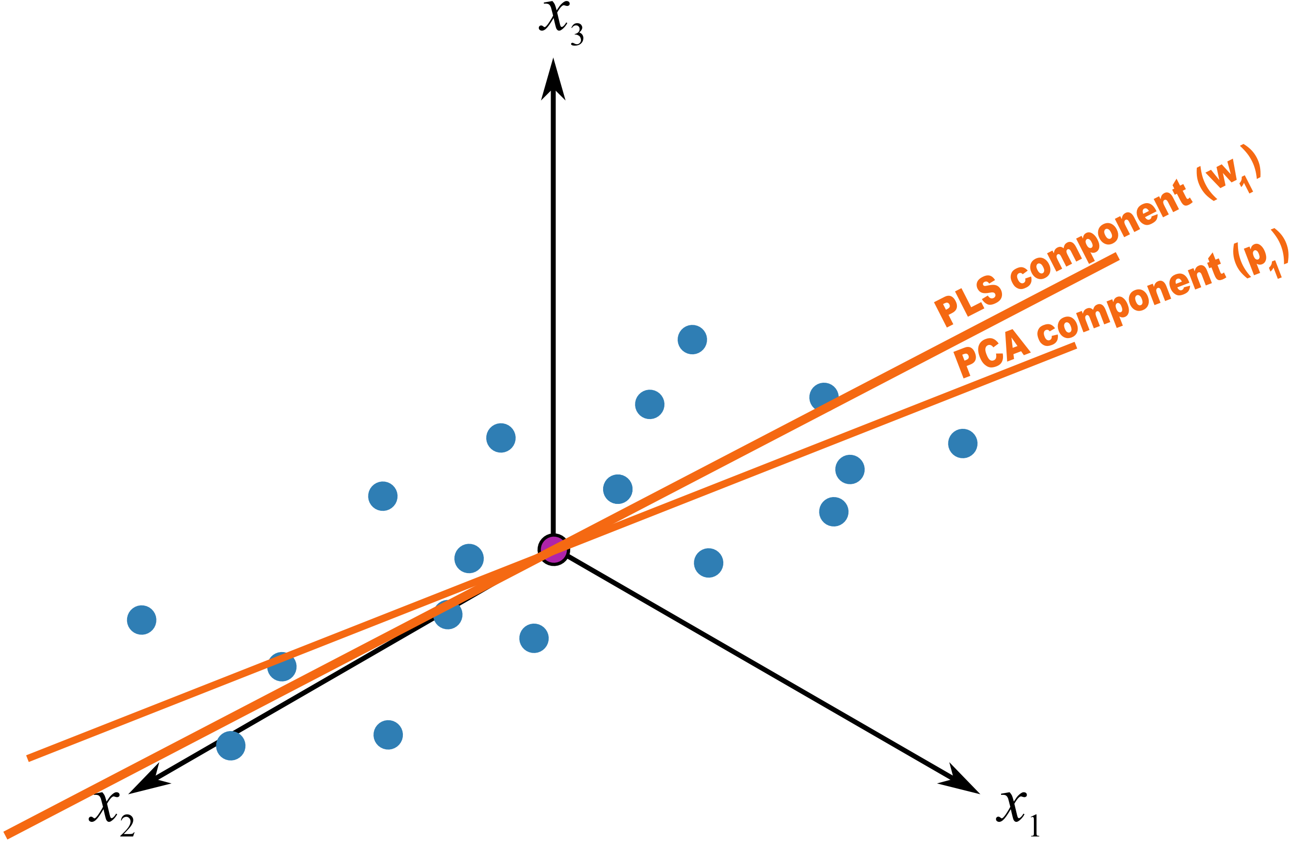
The only difference that must be remembered is that these scores have a different orientation to the PCA scores. As illustrated below, the PCA scores are found so that they only explain the variance in \(\mathbf{X}\); the PLS scores are calculated so that they also explain \(\mathbf{Y}\) and have a maximum relationship between \(\mathbf{X}\) and \(\mathbf{Y}\). Most time these directions will be close together, but not identical.

6.7.6. Interpreting the loadings in PLS

Like with the loadings from PCA, \(\mathbf{p}_a\),we interpret the loadings \(\mathbf{w}_a\) from PLS in the same way. Highly correlated variables have similar weights in the loading vectors and appear close together in the loading plots of all dimensions.

We tend to refer to the PLS loadings, \(\mathbf{w}_a\), as weights; this is for reasons that will be explained soon.

There are two important differences though when plotting the weights. The first is that we superimpose the loadings plots for the \(\mathbf{X}\) and \(\mathbf{Y}\) space simultaneously. This is very powerful, because we not only see the relationship between the \(\mathbf{X}\) variables (from the \(\mathbf{w}\) vectors), we also see the relationship between the \(\mathbf{Y}\) variables (from the \(\mathbf{c}\) vectors), and even more usefully, the relationship between all these variables.

This agrees again with our (engineering) intuition that the \(\mathbf{X}\) and \(\mathbf{Y}\) variables are from the same system; they have been, somewhat arbitrarily, put into different blocks. The variables in \(\mathbf{Y}\) could just have easily been in \(\mathbf{X}\), but they are usually not available due to time delays, expense of measuring them frequently, etc. So it makes sense to consider the \(\mathbf{w}_a\) and \(\mathbf{c}_a\) weights simultaneously.

The second important difference is that we don’t actually look at the \(\mathbf{w}\) vectors directly, we consider rather what is called the \(\mathbf{r}\) vector, though much of the literature refers to it as the \(\mathbf{w*}\) vector (w-star). The reason for the change of notation from existing literature is that \(\mathbf{w*}\) is confusingly similar to the multiplication operator (e.g. \(\mathbf{w*c}\): is frequently confused by newcomers, whereas \(\mathbf{r:c}\) would be cleaner). The \(\mathbf{w*}\) notation gets especially messy when adding other superscript and subscript elements to it. Further, some of the newer literature on PLS, particularly SIMPLS, uses the \(\mathbf{r}\) notation.

The \(\mathbf{r}\) vectors show the effect of each of the original variables, in undeflated form, rather that using the \(\mathbf{w}\) vectors which are the deflated vectors. This is explained next.