6.5.2. Geometric explanation of PCA
We refer to a \(K\)-dimensional space when referring to the data in \(\mathbf{X}\). We will start by looking at the geometric interpretation of PCA when \(\mathbf{X}\) has 3 columns, in other words a 3-dimensional space, using measurements: \([x_1, x_2, x_3]\).
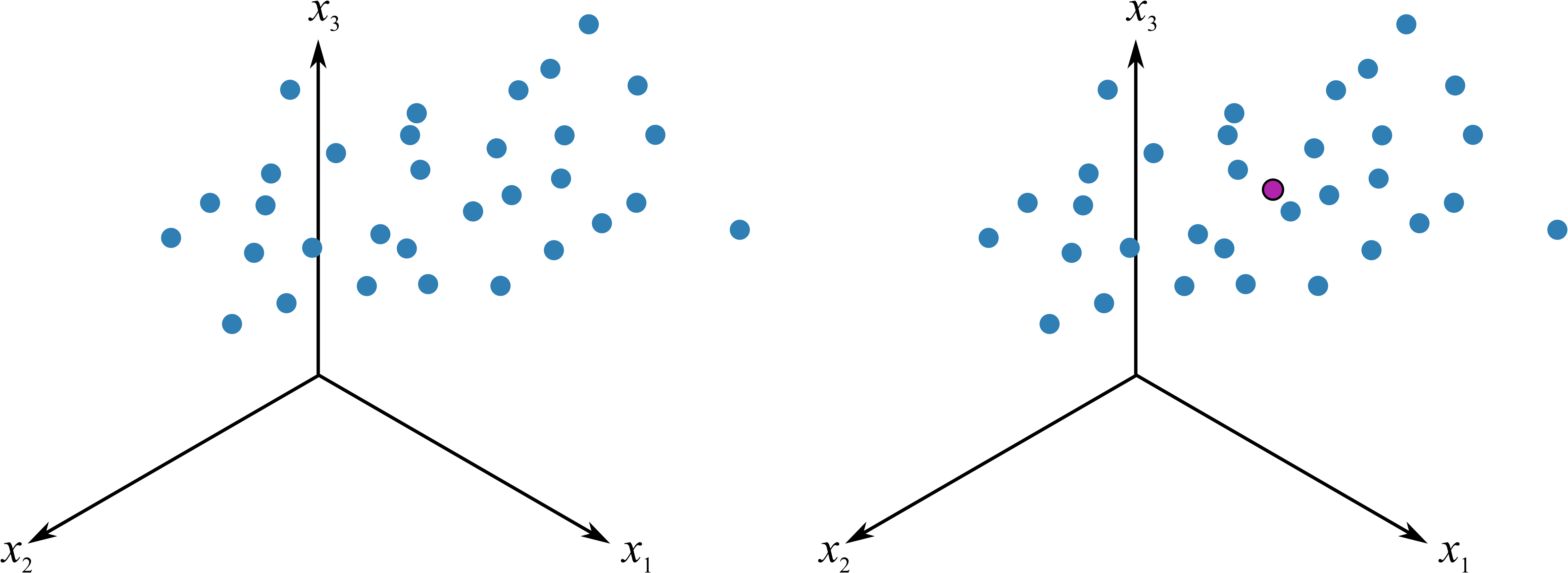
The raw data in the cloud swarm show how the 3 variables move together. The first step in PCA is to move the data to the center of the coordinate system. This is called mean-centering and removes the arbitrary bias from measurements that we don’t wish to model. We also scale the data, usually to unit-variance. This removes the fact that the variables are in different units of measurement. Additional discussion on centering and scaling is in the section on data preprocessing.
After centering and scaling we have moved our raw data to the center of the coordinate system and each variable has equal scaling.
The best-fit line is drawn through the swarm of points. The more correlated the original data, the better this line will explain the actual values of the observed measurements. This best-fit line will best explain all the observations with minimum residual error. Another, but equivalent, way of expressing this is that the line goes in the direction of maximum variance of the projections onto the line. Let’s take a look at what that phrase means.
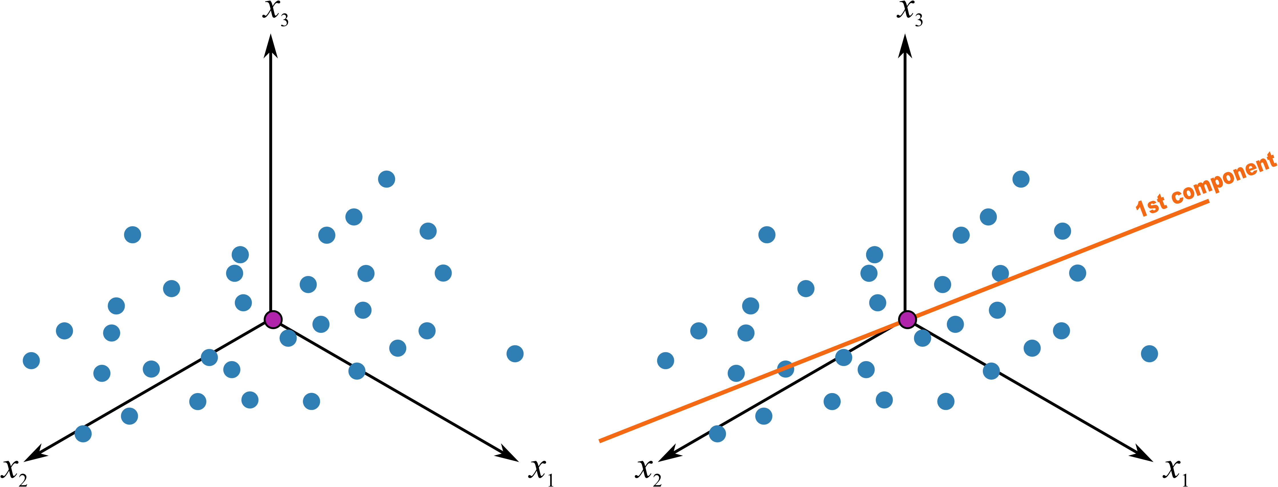
When the direction of the best-fit line is found we can mark the location of each observation along the line. We find the 90 degree projection of each observation onto the line (see the next illustration). The distance from the origin to this projected point along the line is called the score. Each observation gets its own score value. When we say the best-fit line is in the direction of maximum variance, what we are saying is that the variance of these scores will be maximal. (There is one score for each observation, so there are \(N\) score values; the variance of these \(N\) values is at a maximum). Notice that some score values will be positive and others negative.
After we have added this best-fit line to the data, we have calculated the first principal component, also called the first latent variable. Each principal component consists of two parts:
The direction vector that defines the best-fit line. This is a \(K\)-dimensional vector that tells us which direction that best-fit line points, in the \(K\)-dimensional coordinate system. We call this direction vector \(\mathbf{p}_1\), it is a \(K \times 1\) vector. This vector starts at the origin and moves along the best-fit line. Since vectors have both magnitude and direction, we chose to rescale this vector so that it has magnitude of exactly 1, making it a unit-vector.
The collection of \(N\) score values along this line. We call this our score vector, \(\mathbf{t}_1\), and it is an \(N \times 1\) vector.
The subscript of “1” emphasizes that this is the first latent variable.
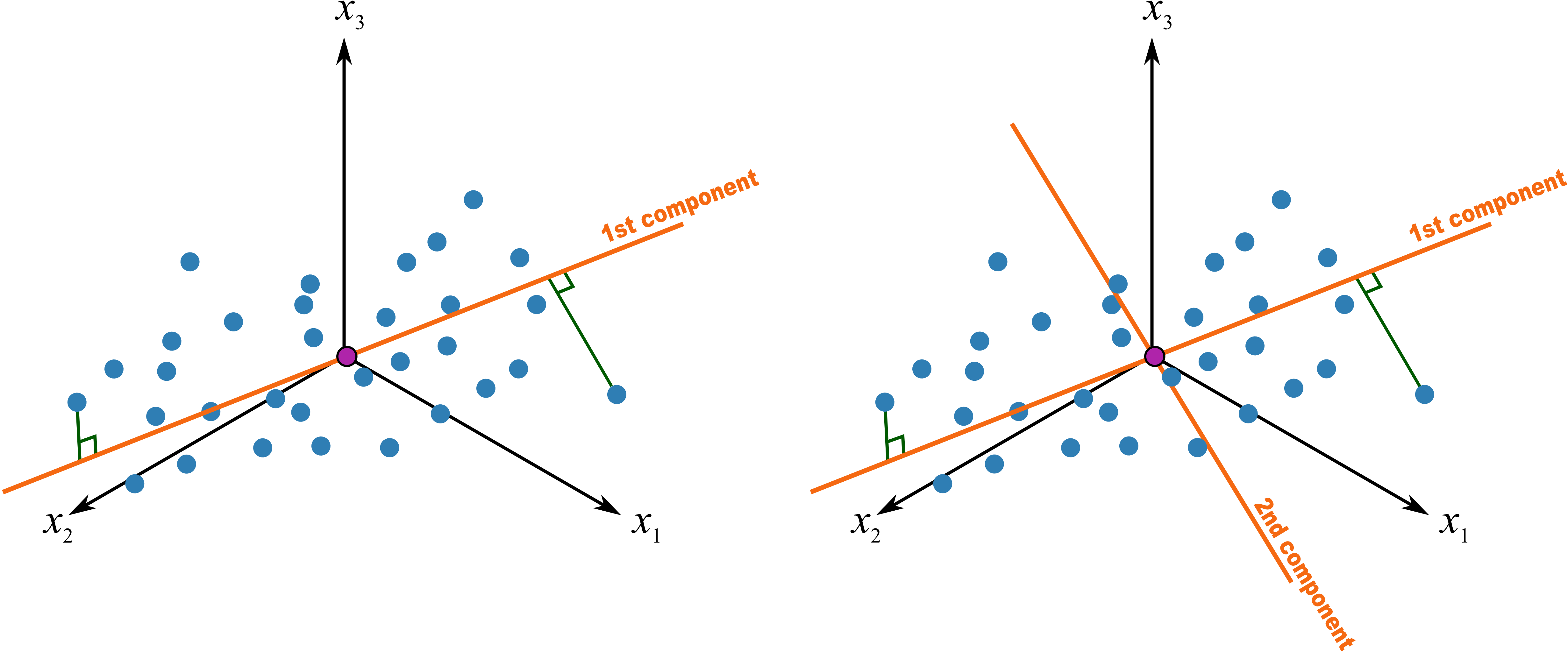
This first principal component is fixed and we now add a second component to the system. We find the second component so that it is perpendicular to the first component’s direction. Notice that this vector also starts at the origin, and can point in any direction as long as it remains perpendicular to the first component. We keep rotating the second component’s direction vector around until we find a direction that gives the greatest variance in the score values when projected on this new direction vector.
What that means is that once we have settled on a direction for the second component, we calculate the scores values by perpendicularly projecting each observation towards this second direction vector. The score values for the second component are the locations along this line. As before, there will be some positive and some negative score values. This completes our second component:
This second direction vector, called \(\mathbf{p}_2\), is also a \(K \times 1\) vector. It is a unit vector that points in the direction of next-greatest variation.
The scores (distances), collected in the vector called \(\mathbf{t}_2\), are found by taking a perpendicular projection from each observation onto the \(\mathbf{p}_2\) vector.
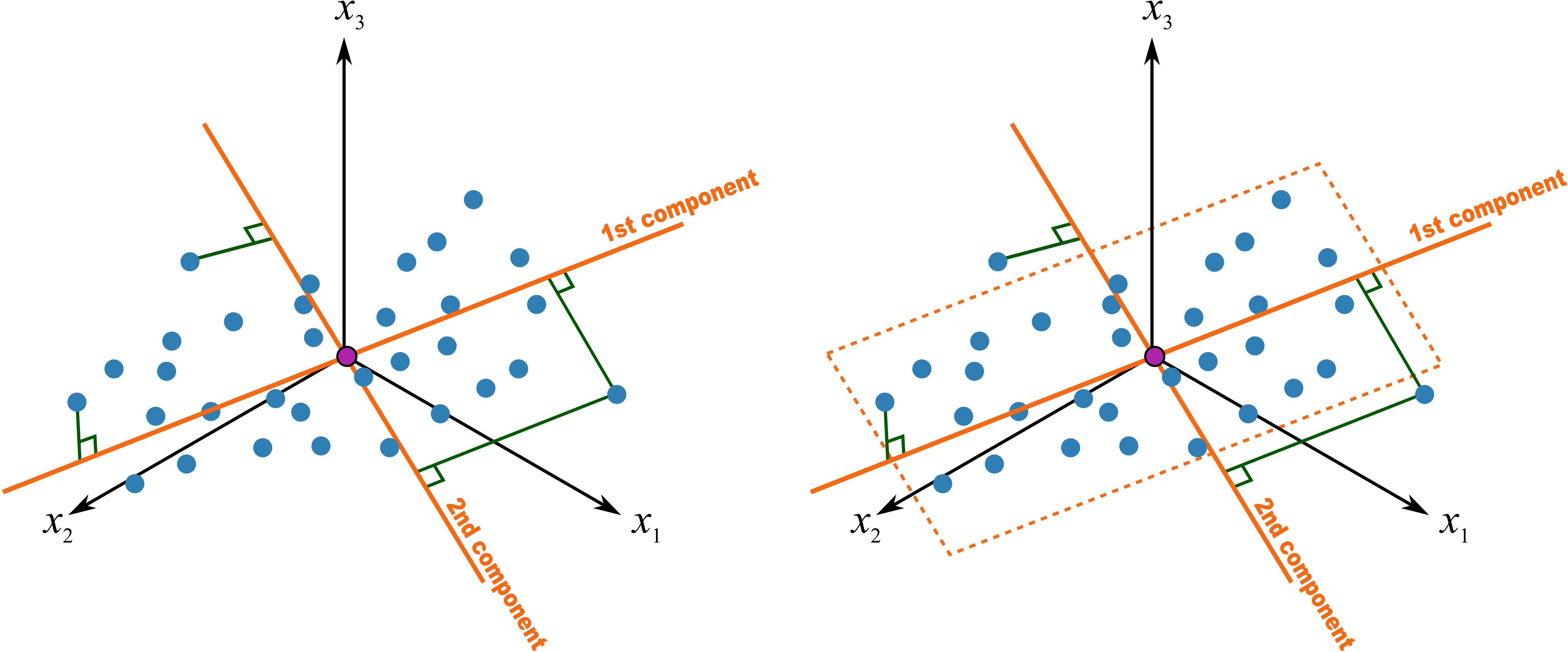
Notice that the \(\mathbf{p}_1\) and \(\mathbf{p}_2\) vectors jointly define a plane. This plane is the latent variable model with two components. With one component the latent variable model is just a line, with two components, the model is a plane, and with 3 or more components, the model is defined by a hyperplane. We will use the letter \(a\) to identify the number of components. The PCA model is said to have \(A\) components, or \(A\) latent variables, where \(a = 1, 2, 3, \ldots A\).
This hyperplane is really just the best approximation we can make of the original data. The perpendicular distance from each point onto the plane is called the residual distance or residual error. So what a principal component model does is break down our raw data into two parts:
a latent variable model (given by vectors \(\mathbf{p}\) and \(\mathbf{t}\)), and
a residual error.
A principal component model is one type of latent variable model. A PCA model is computed in such a way that the latent variables are oriented in the direction that gives greatest variance of the scores. There are other latent variable models, but they are computed with different objectives.