2.12. Testing for differences and similarity
These sort of questions often arise in data analysis:
We want to change to a cheaper material, B. Does it work as well as A?
We want to introduce a new catalyst B. Does it improve our product properties over the current catalyst A?
Either we want to confirm things are statistically the same, or confirm they have changed. Notice that in both the above cases we are testing the population mean (location). Has the mean shifted or is it the same? There are also tests for changes in variance (spread), which we will cover. We will work with an example throughout this section.
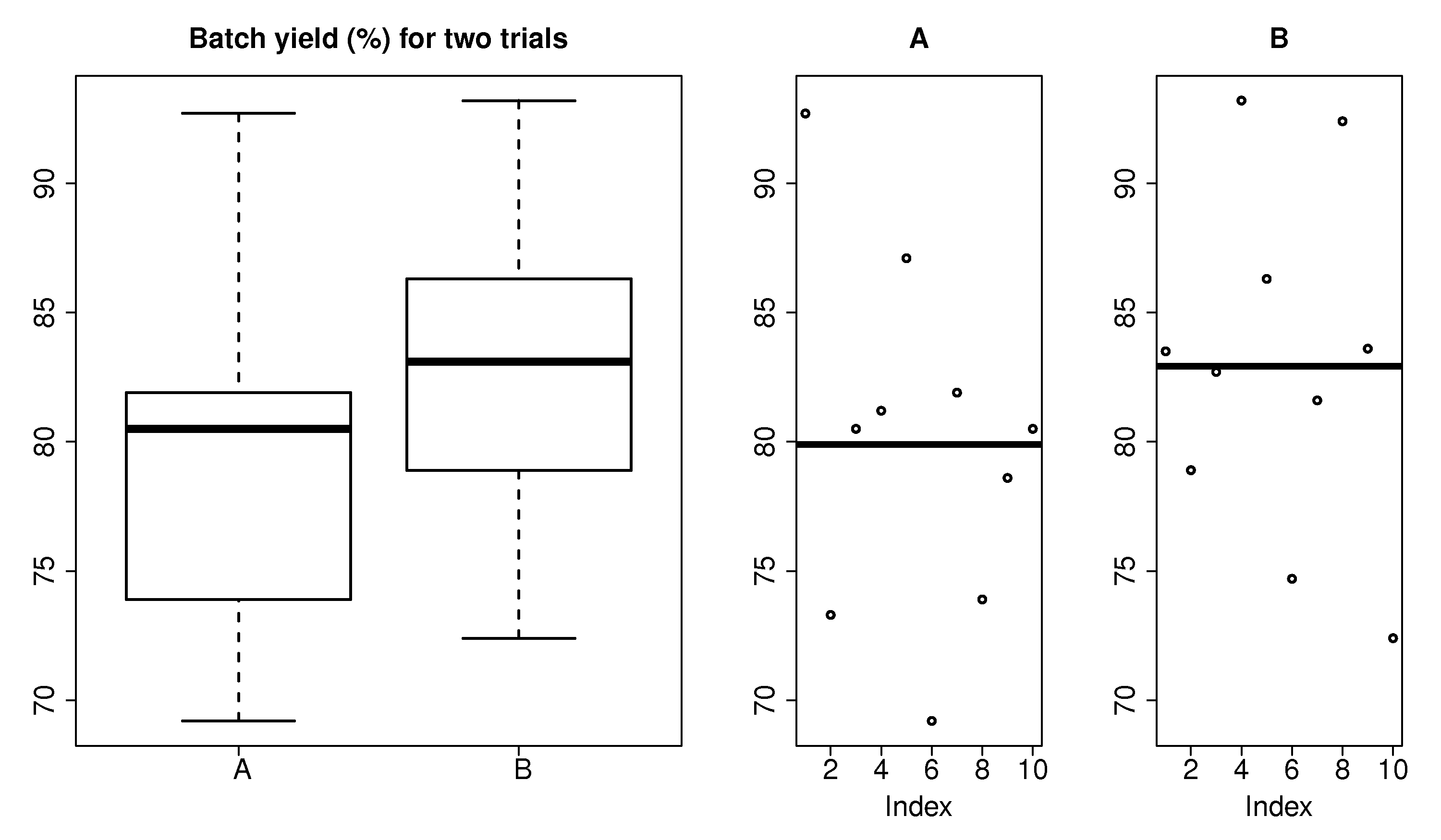
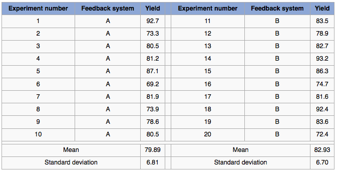
Example: A process operator needs to verify that a new form of feedback control on the batch reactor leads to improved yields. Yields under the current control system, A, are compared with yields under the new system, B. The last ten runs with system A are compared to the next 10 sequential runs with system B. The data are shown in the table, and shown in graphical form as well. (Note that the box plot uses the median, while the plots on the right show the mean.)
We address the question of whether or not there was a significant difference between system A and B. A significant difference means that when system B is compared to a suitable reference, that we can be sure that the long run implementation of B will lead, in general, to a different yield (%). We want to be sure that any change in the 10 runs under system B were not only due to chance, because system B will cost us $100,000 to install, and $20,000 in annual software license fees.
Note: those with a traditional statistical background will recognize this section as one-sided hypothesis tests. We will only consider tests for a significant increase or decrease, i.e. one-sided tests, in this section. We use confidence intervals, rather than hypothesis tests; the results are exactly the same. Arguably the confidence interval approach is more interpretable, since we get a bound, rather that just a clear-cut yes/no answer.
There are two main ways to test for a significant increase or significant decrease.
2.12.1. Comparison to a long-term reference set
Continuing the above example we can compare the past 10 runs from system B with the 10 runs from system A. The average difference between these runs is \(\overline{x}_B - \overline{x}_A = 82.93 - 79.89 = 3.04\) units of improved yield. Now, if we have a long-term reference data set available, we can compare if any 10 historical, sequential runs from system A, followed by another 10 historical, sequential runs under system A had a difference that was this great. If not, then we know that system B leads to a definite improvement, not likely to be caused by chance alone.
Here’s the procedure:
Imagine that we have 300 historical data points from this system, tabulated in time order: yield from batch 1, 2, 3 … (the data are available on the website).
Calculate the average yields from batches 1 to 10. Then calculate the average yield from batches 11 to 20. Notice that this is exactly like the experiment we performed when we acquired data for system B: two groups of 10 batches, with the groups formed from sequential batches.
Now subtract these two averages: (group average 11 to 20) minus (group average 1 to 10).
Repeat steps 2 and 3, but use batches 2 to 11 and 12 to 21. Repeat until all historical batch data are used up, i.e. batches 281 to 290 and 291 to 300. The plot below can be drawn, one point for each of these difference values.
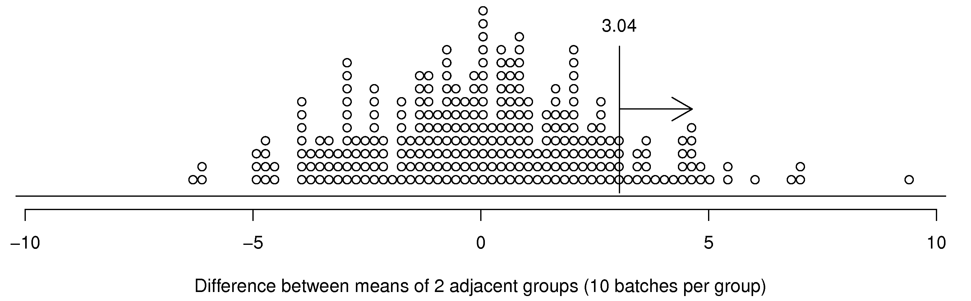
The vertical line at 3.04 is the difference value recorded between system B and system A. From this we can see that historically, there were 31 out of 281 batches, about 11% of historical data, that had a difference value of 3.04 or greater. So there is a 11% probability that system B was better than system A purely by chance, and not due to any technical superiority. Given this information, we can now judge, if the improved control system will be economically viable and judge, based on internal company criteria, if this is a suitable investment, also considering the 11% risk that our investment will fail.
Notice that no assumption of independence or any form of distributions was required for this work! The only assumption made is that the historical data are relevant. We might know this if, for example, no substantial modification was made to the batch system for the duration over which the 300 samples were acquired. If however, a different batch recipe were used for sample 200 onwards, then we may have to discard those first 200 samples: it is not fair to judge control system B to the first 200 samples under system A, when a different operating procedure was in use.
So to summarize: we can use a historical data set if it is relevant. And there are no assumptions of independence or shape of the distribution, e.g. a normal distribution.
In fact, for this example, the data were not independent, they were autocorrelated. There was a relationship from one batch to the next: \(x[k] = \phi x[k-1] + a[k]\), with \(\phi = -0.3\), and \(a[k] \sim \mathcal{N}\left(\mu=0, \sigma^2=6.7^2\right)\). As an aside you can simulate your own set of autocorrelated data using this R code:
We can visualize this autocorrelation by plotting the values of \(x[k]\) against \(x[k+1]\):
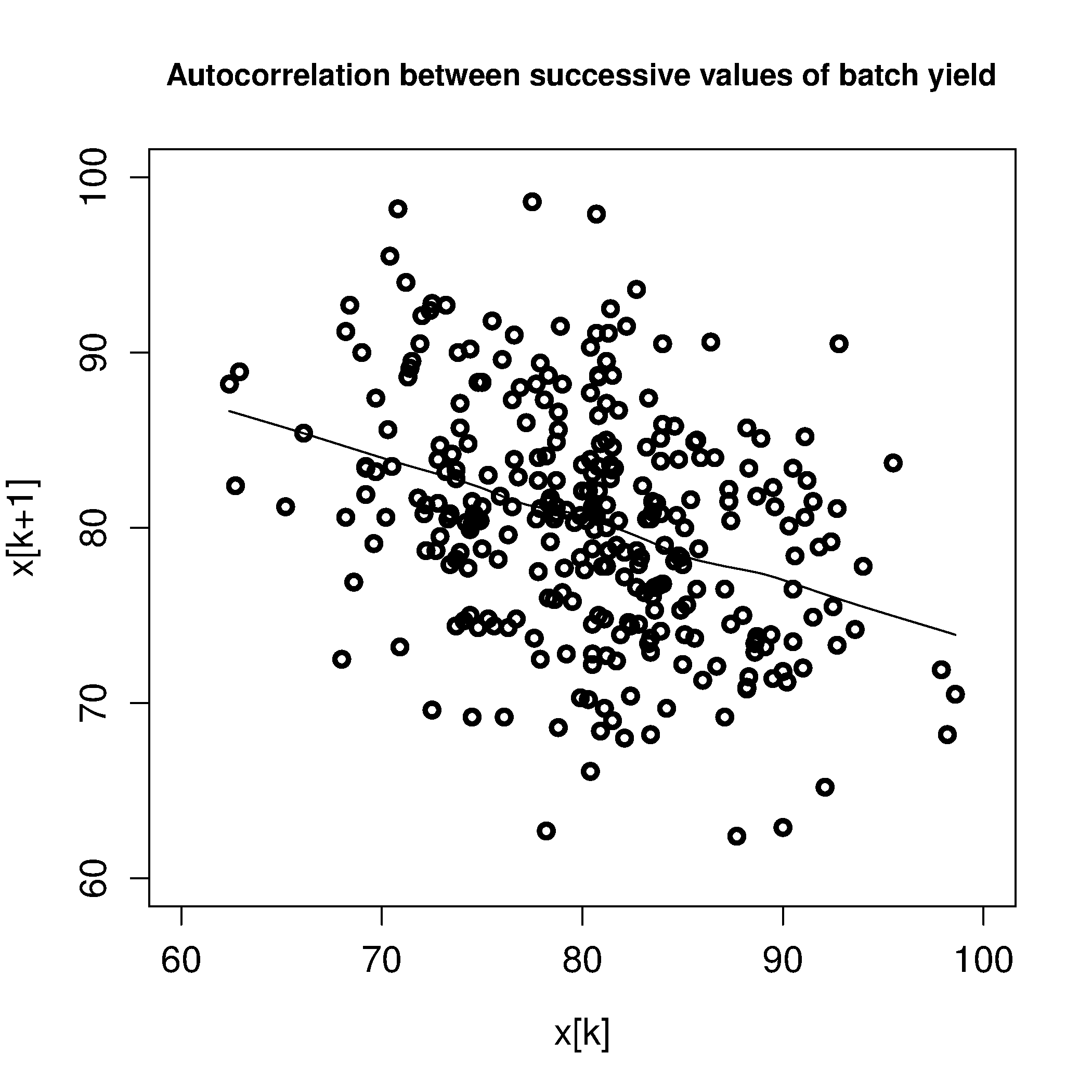
We can immediately see the data are not independent, because the slope is non-zero.
2.12.2. Comparison when a reference set is not available
A reference data set may not always be available; we may only have the data from the 20 experimental runs (10 from system A and 10 from B) and nothing else. We can proceed to compare the data, but we will require a strong assumption of random sampling (independence), which is often not valid in engineering data sets. Fortunately, engineering data sets are usually large - we are good at collecting data - so the methodology in the preceding section on using a reference set, is greatly preferred, when possible.
How could the assumption of independence (random sampling) be made more realistically? How is the lack of independence detrimental? We show below that the assumption of independence is made twice: the samples within group A and B must be independent; furthermore, the samples between the groups should be independent. But first we have to understand why the assumption of independence is required, by understanding the usual approach for estimating if differences are significant or not.
The usual approach for assessing if the difference between \(\overline{x}_B - \overline{x}_A\) is significant follows this approach:
Assume the data for sample A and sample B have been independently sampled from their respective populations.
Assume the data for sample A and sample B have the same population variance, \(\sigma_A = \sigma_B = \sigma\) (there is a test for this, see the next section).
Let the sample A have population mean \(\mu_A\) and sample B have population mean \(\mu_B\).
From the central limit theorem (this is where the assumption of independence of the samples within each group comes), we know that:
\begin{alignat*}{2} \mathcal{V}\left\{\overline{x}_A\right\} = \frac{\sigma^2_A}{n_A} &\qquad\qquad & \mathcal{V}\left\{\overline{x}_B\right\} = \frac{\sigma^2_B}{n_B} \end{alignat*}Assuming independence again, but this time between groups, this implies the average of each sample group is independent, i.e. \(\overline{x}_A\) and \(\overline{x}_B\) are independent of each other. This allows us to write:
(1)¶\[ \mathcal{V}\left\{\overline{x}_B - \overline{x}_A\right\} = \frac{\sigma^2}{n_A} + \frac{\sigma^2}{n_B} = \sigma^2 \left(\frac{1}{n_A} + \frac{1}{n_B}\right)\]Using the central limit theorem, even if the samples in A and the samples in B are non-normal, the sample averages \(\overline{x}_A\) and \(\overline{x}_B\) will be more normal as the sample size becomes progressively larger. So the difference between these means will also be more normal: \(\overline{x}_B - \overline{x}_A\). Now express this difference in the form of a \(z\)-deviate (standard form):
(2)¶\[ z = \frac{(\overline{x}_B - \overline{x}_A) - (\mu_B - \mu_A)}{\sqrt{\sigma^2 \left(\displaystyle \frac{1}{n_A} + \frac{1}{n_B}\right)}}\]We could ask, what is the probability of seeing a \(z\) value from equation (2) of that magnitude? Recall that this \(z\)-value is the equivalent of \(\overline{x}_B - \overline{x}_A\), expressed in deviation form, and we are interested if this difference is due to chance. So we should ask, what is the probability of getting a value of \(z\) greater than this, or smaller that this, depending on the case?
The only question remains is what is a suitable value for \(\sigma\)? As we have seen before, when we have a large enough reference set, then we can use the value of \(\sigma\) from the historical data, called an external estimate. Or we can use an internal estimate of spread; both approaches are discussed below.
Now we know the approach required, using the above 6 steps, to determine if there was a significant difference. And we know the assumptions that are required: normally distributed and independent samples. But how can we be sure our data are independent? This is the most critical aspect, so let’s look at a few cases and discuss, then we will return to our example and calculate the \(z\)-values with both an external and internal estimate of spread.
Discuss whether these experiments would lead to independent data or not, and how we might improve the situation.
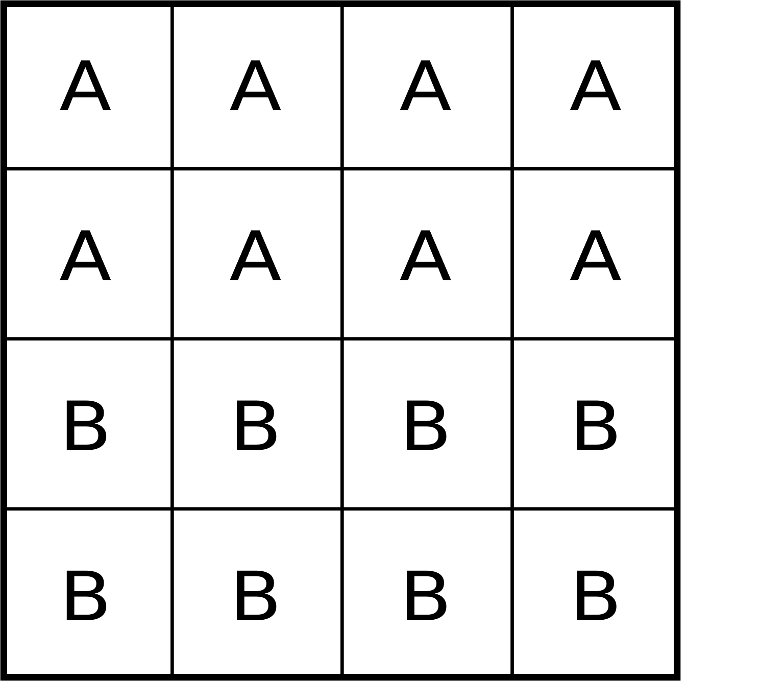
We are testing a new coating to repel moisture. The coating is applied to packaging sheets that are already hydrophobic, however this coating enhances the moisture barrier property of the sheet. In the lab, we take a large packaging sheet and divide it into 16 blocks. We coat the sheet as shown in the figure and then use the \(n_A=8\) and \(n_B=8\) values of hydrophobicity to judge if coating B is better than coating A.
Some problems with this approach:
The packaging sheet to which the new coating is applied may not be uniform. The sheet is already hydrophobic, but the hydrophobicity is probably not evenly spread over the sheet, nor are any of the other physical properties of the sheet. When we measure the moisture repelling property with the different coatings applied, we will not have an accurate measure of whether coating A or B worked better. We must randomly assign blocks A and B on the packaging sheet.
Even so, this may still be inadequate, because what if the packaging sheet selected has overly high or low hydrophobicity (i.e. it is not representative of regular packaging sheets). What should be done is that random packaging sheets should be selected, and they should be selected across different lots from the sheet supplier (sheets within one lot are likely to be more similar than between lots). Then on each sheet we apply coatings A and B, in a random order on each sheet.
It is tempting to apply coating A and B to one half of the various sheets and measure the difference between the moisture repelling values from each half. It is tempting because this approach would cancel out any base variation between difference sheets, as long as that variation is present across the entire sheet. Then we can go on to assess if this difference is significant.
There is nothing wrong with this methodology, however, there is a different, specific test for paired data, covered in a later section. If you use the above test, you violate the assumption in step 5, which requires that \(\overline{x}_A\) and \(\overline{x}_B\) be independent. Values within group A and B are independent, but not their sample averages, because you cannot calculate \(\overline{x}_A\) and \(\overline{x}_B\) independently.
We are testing an alternative, cheaper raw material in our process, but want to be sure our product’s final properties are unaffected. Our raw material dispensing system will need to be modified to dispense material B. This requires the production line to be shut down for 15 hours while the new dispenser, lent from the supplier, is installed. The new supplier has given us 8 representative batches of their new material to test, and each test will take 3 hours. We are inclined to run these 8 batches over the weekend: set up the dispenser on Friday night (15 hours), run the tests from Saturday noon to Sunday noon, then return the line back to normal for Monday’s shift. How might we violate the assumptions required by the data analysis steps above when we compare 8 batches of material A (collected on Thursday and Friday) to the 8 batches from material B (from the weekend)? What might we do to avoid these problems?
The 8 tests are run sequentially, so any changes in conditions between these 8 runs and the 8 runs from material A will be confounded (confused) in the results. List some actual scenarios how confounding between the weekday and weekend experiments occur:
For example, the staff running the equipment on the weekend are likely not the same staff that run the equipment on weekdays.
The change in the dispenser may have inadvertently modified other parts of the process, and in fact the dispenser itself might be related to product quality.
The samples from the tests will be collected and only analyzed in the lab on Monday, whereas the samples from material A are usually analyzed on the same day: that waiting period may degrade the sample.
This confounding with all these other, potential factors means that we will not be able to determine whether material B caused a true difference, or whether it was due to the other conditions.
It is certainly expensive and impractical to randomize the runs in this case. Randomization would mean we randomly run the 16 tests, with the A and B chosen in random order, e.g.
A B A B A A B B A A B B B A B A. This particular randomization sequence would require changing the dispenser 9 times.One suboptimal sequence of running the system is
A A A A B B B B A A A A B B B B. This requires changing the dispenser 4 times (one extra change to get the system back to material A). We run each (A A A A B B B B) sequence on two different weekends, changing the operating staff between the two groups of 8 runs, making sure the sample analysis follows the usual protocols: so we reduce the chance of confounding the results.
Randomization might be expensive and time-consuming in some studies, but it is the insurance we require to avoid being misled. These two examples demonstrate this principle: block what you can and randomize what you cannot. We will review these concepts again in the design and analysis of experiments section. If the change being tested is expected to improve the process, then we must follow these precautions to avoid a process upgrade/modification that does not lead to the expected improvement; or the the converse - a missed opportunity of implementing a change for the better.
2.12.2.1. External and internal estimates of spread
So to recap the progress so far, we are aiming to test if there is a significant, long-term difference between two systems: A and B. We showed the most reliable way to test this difference is to compare it with a body of historical data, with the comparison made in the same way as when the data from system A and B were acquired; this requires no additional assumptions, and even allows one to run experiments for system B in a non-independent way.
But, because we do not always have a large and relevant body of data available, we can calculate the difference between A and B and test if this difference could have occurred by chance alone. For that we use equation (2), but we need an estimate of the spread, \(\sigma\).
External estimate of spread
The question we turn to now is what value to use for \(\sigma\) in equation (2). We got to that equation by assuming we have no historical, external data. But what if we did have some external data? We could at least estimate \(\sigma\) from that. For example, the 300 historical batch yields has \(\sigma = 6.61\):
Check the probability of obtaining the \(z\)-value in (2) by using the hypothesis that the value \(\mu_B - \mu_A = 0\). In other words we are making a statement, or a test of significance. Then we calculate this \(z\)-value and its associated cumulative probability:
The probability of seeing a \(z\)-value from \(-\infty\) up to 1.03 is 84.8% (use the pnorm(1.03) function in R). But we are interested in the probability of obtaining a \(z\)-value larger than this. Why? Because \(z=0\) represents no improvement, and a value of \(z<0\) would mean that system B is worse than system A. So what are the chances of obtaining \(z=1.03\)? It is (100-84.8)% = 15.2%, which means that system B’s performance could have been obtained by pure luck in 15.2% of cases.
We interpret this number of “15.2%” in the summary section, but let’s finally look at what happens if we have no historical data - then we generate an internal estimate of \(\sigma\) from the 20 experimental runs alone.
Internal estimate of spread
The sample variance from each system was \(s_A^2 = 6.81^2\) and \(s_B^2 = 6.70^2\), and in this case it happened that \(n_A = n_B = 10\), although the sample sizes do not necessarily have to be the same.
If the variances are comparable (there is a test for that below), then we can calculate a pooled variance, \(s_P^2\), which is a weighted sum of the sampled variances:
Now using this value of \(s_P\) instead of \(\sigma\) in (2):
The probability of obtaining a \(z\)-value greater than this can be calculated as 16.4% using the \(t\)-distribution with 18 degrees of freedom (use 1-pt(1.01, df=18) in R). We use a \(t\)-distribution because an estimate of the variance is used, \(s_p^2\), not a population variance, \(\sigma^2\).
As an aside: we used a normal distribution for the external \(\sigma\) and a \(t\)-distribution for the internal \(s\). Both cases had a similar value for \(z\) (compare \(z = 1.01\) to \(z = 1.03\)). Note however that the probabilities are higher in the \(t\)-distribution’s tails, which means that even though we have similar \(z\)-values, the probability is greater: 16.4% against 15.2%. While this difference is not much from a practical point of view, it illustrates the difference between the \(t\)-distribution and the normal distribution.
The results from this section were achieved by only using the 20 experimental runs, no external data. However, it made some strong assumptions:
The variances of the two samples are comparable, and can therefore be pooled to provide an estimate of \(\sigma\).
The usual assumption of independence within each sample is made (which we know not to be true for many practical engineering cases).
The assumption of independence between the samples is also made (this is more likely to be true in this example, because the first runs to acquire data for A are not likely to affect the runs for system B).
Each sample, A and B, is assumed to be normally distributed.
2.12.2.2. Summary and comparison of methods
Let’s compare the 3 estimates. Recall our aim is to convince ourself/someone that system B will have better long-term performance than the current system A.
If we play devil’s advocate, our null hypothesis is that system B has no effect. Then it is up to us to prove, convincingly, that the change from A to B has a systematic, permanent effect. That is what the calculated probabilities represent :, the probability of us being wrong.
Using only reference data: 11% (about 1 in 10)
Using the 20 experimental runs, but an external estimate of \(\sigma\): 15.2% (about 1 in 7)
Using the 20 experimental runs only, no external data: 16.4% (about 1 in 6)
The reference data method shows that the trial with 10 experiments using system B could have actually been taken from the historical data with a chance of 11%. A risk adverse company may want this number to be around 5%, or as low as 1% (1 in 100), which essentially guarantees the new system will have better performance.
When constructing the reference set, we have to be sure the reference data are appropriate. Were the reference data acquired under conditions that were similar to the time in which data from system B were acquired? In this example, they were, but in practice, careful inspection of plant records must be made to verify this.
The other two methods mainly use the experimental data, and provide essentially the same answer in this case study, though that is not always the case. The main point here is that our experimental data are usually not independent. However, by careful planning, and expense, we can meet the requirement of independence by randomizing the order in which we acquire the data. Randomization is the insurance (cost) we pay so that we do not have to rely on a large body of prior reference data. But in some cases it is not possible to randomize, so blocking is required. More on blocking in the design of experiments section.