5.8.1. Using two levels for two or more factors
Let’s take a look at the mechanics of factorial designs by using our previous example where the conversion, \(y\), is affected by two factors: temperature, \(T\), and substrate concentration, \(S\).
The range over which they will be varied is given in the table. This range was identified by the process operators as being sufficient to actually show a difference in the conversion, but not so large as to move the system to a totally different operating regime (that’s because we will fit a linear model to the data).
Factor
Low level, \(-\)
High level, \(+\)
Temperature, \(T\)
338 K
354 K
Substrate level, \(S\)
1.25 g/L
1.75 g/L
Write down the factors that will be varied: \(T\) and \(S\).
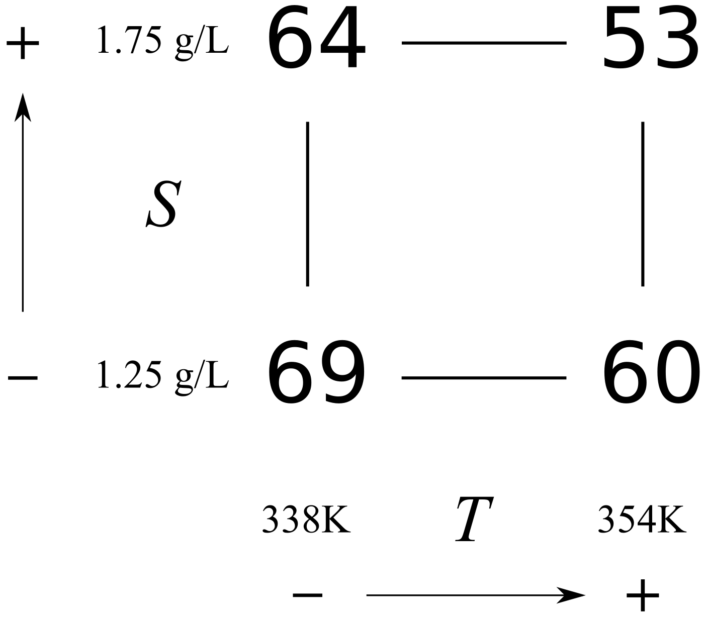
Write down the coded runs in standard order, also called Yates order, which alternates the sign of the first variable the fastest and the last variable the slowest. By convention we start all runs at their low levels and finish off with all factors at their high levels. There will be \(2^k\) runs, where \(k\) is the number of variables in the design and the \(2\) refers to the number of levels for each factor. In this case, \(2^2 = 4\) experiments (runs). We perform the actual experiments in random order, but always write the table in this standard order.
Experiment
\(T\) [K]
\(S\) [g/L]
1
\(-\)
\(-\)
2
\(+\)
\(-\)
3
\(-\)
\(+\)
4
\(+\)
\(+\)
Add an additional column to the table for the response variable. The response variable is a quantitative value, \(y\), which in this case is the conversion measured as a percentage.
Experiment
Order
\(T\) [K]
\(S\) [g/L]
\(y\) [%]
1
3
\(-\)
\(-\)
69
2
2
\(+\)
\(-\)
60
3
4
\(-\)
\(+\)
64
4
1
\(+\)
\(+\)
53
Experiments were performed in random order; in this case, we happened to run experiment 4 first and experiment 3 last.
For simple systems you can visualize the design and results as shown in the following figure. This is known as a cube plot.
5.8.2. Analysis of a factorial design: main effects
The first step is to calculate the main effect of each variable. The effects are considered, by convention, to be the difference from the high level to the low level. So the interpretation of a main effect is by how much the outcome, \(y\), is adjusted when changing the variable.
Consider the two runs where \(S\) is at the \(-\) level for both experiments 1 and 2. The only change between these two runs is the temperature, so the temperature effect is \(\Delta T_{S-} = 60-69 = -9\%\,\,\text{per}\,\,(354-338)~\text{K}\), that is, a \(-9\%\) change in the conversion outcome per \(+16~\text{K}\) change in the temperature.
Runs 3 and 4 both have \(S\) at the \(+\) level. Again, the only change is in the temperature: \(\Delta T_{S+} = 53-64 = -11\%\) per \(+16~\text{K}\). So we now have two temperature effects, and the average of them is a \(-10\%\) change in conversion per \(+16~\text{K}\) change in temperature.
We can perform a similar calculation for the main effect of substrate concentration, \(S\), by comparing experiments 1 and 3: \(\Delta S_{T-} = 64-69 = -5\%\,\,\text{per}\,\,0.5\,\text{g/L}\), while experiments 2 and 4 give \(\Delta S_{T+} = 53-60 = -7\%\) per \(0.5\,\text{g/L}\). So the average main effect for \(S\) is a \(-6\%\) change in conversion for every \(0.5\,\text{g/L}\) change in substrate concentration. You should use the following graphical method when calculating main effects from a cube plot by hand.
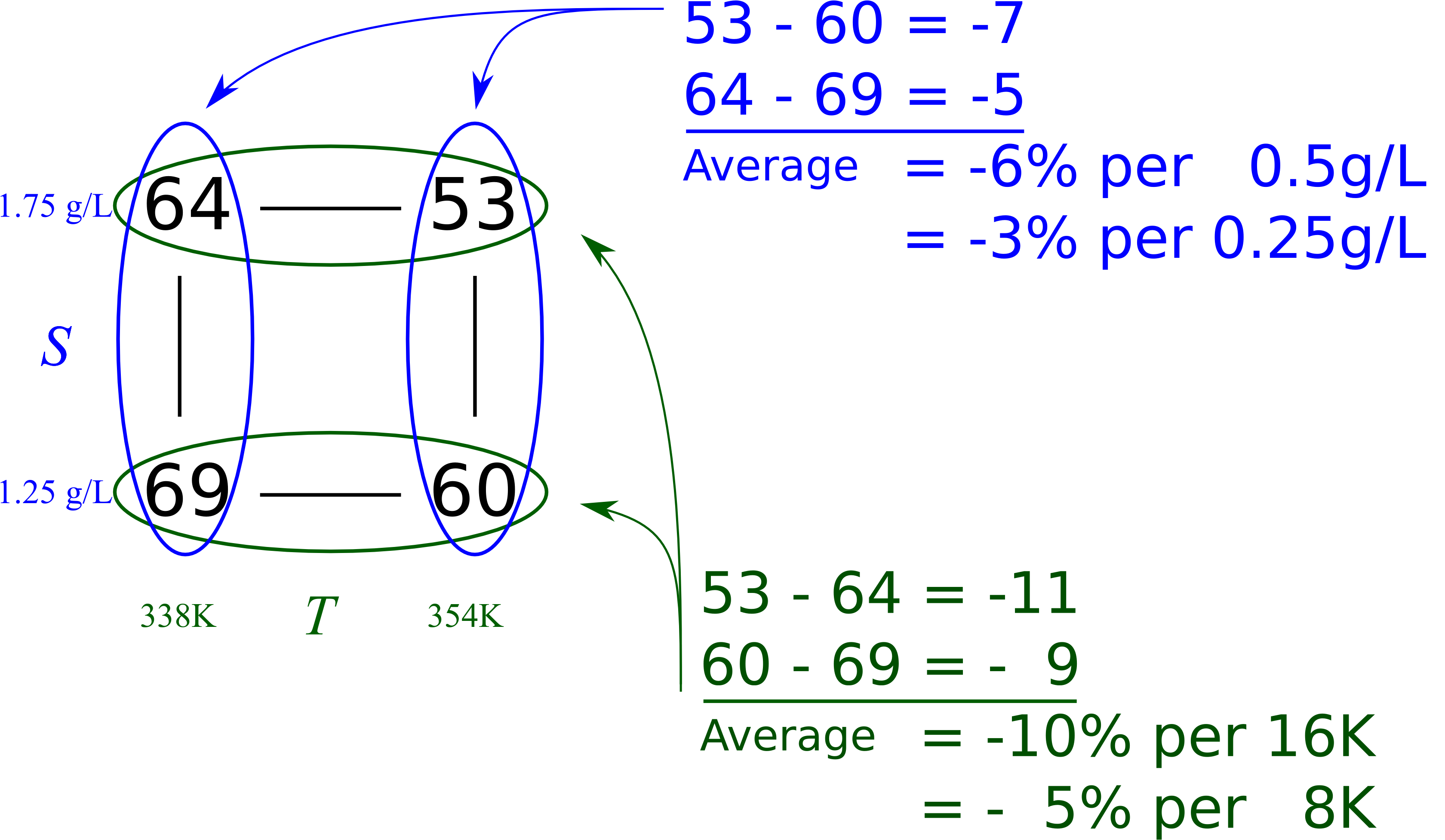
This visual summary is a very effective method of seeing how the system responds to the two variables. We can see the gradients in the system and the likely region where we can perform the next experiments to improve the bioreactor’s conversion.
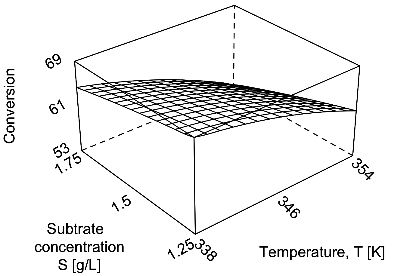
The following surface plot illustrates the true, but unknown, surface from which our measurements are taken. Notice the slight curvature on the edges of each face. The main effects estimated above are a linear approximation of the conversion over the region spanned by the factorial.
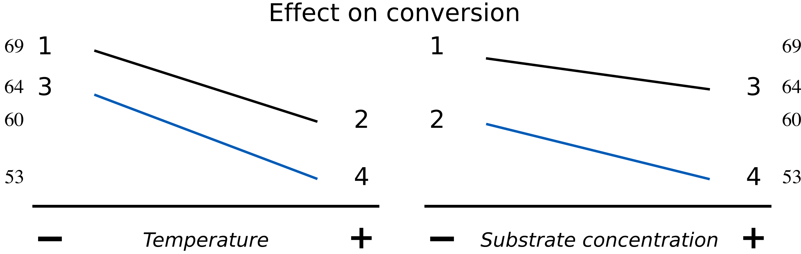
An interaction plot is an alternative way to visualize these main effects. Use this method when you don’t have computer software to draw the surfaces. [We saw this earlier in the visualization section]. We will discuss interaction plots more in the next section. Here is an illustration of one such plot for a system with little interaction.
5.8.3. Analysis of a factorial design: interaction effects
We expect in many real systems that the main effect of temperature, \(T\), for example, is different at other levels of substrate concentration, \(S\). It is quite plausible for a bioreactor system that the main temperature effect on conversion is much greater if the substrate concentration, \(S\), is also high, while at low values of \(S\), the temperature effect is smaller.
We call this result an interaction, when the effect of one factor is different at different levels of the other factors. Let’s give a practical, everyday example: assume your hands are covered with dirt or oil. We know that if you wash your hands with cold water, it will take longer to clean them than washing with hot water. So let factor A be the temperature of the water; factor A has a significant effect on the time taken to clean your hands.
Consider the case when washing your hands with cold water. If you use soap with cold water, it will take less time to clean your hands than if you did not use soap. It is clear that factor B, the categorical factor of using no soap vs some soap, will reduce the time to clean your hands.
Now consider the case when washing your hands with hot water. The time taken to clean your hands with hot water when you use soap is greatly reduced, far faster than any other combination. We say there is an interaction between using soap and the temperature of the water. This is an example of an interaction that works to help us reach the objective faster.
The effect of warm water enhances the effect of soap. Conversely, the effect is soap is enhanced by using warm water. So symmetry means that if soap interacts with water temperature, then we also know that water temperature interacts with soap.
In summary, interaction means the effect of one factor depends on the level of the other factor. In this example, that implies the effect of soap is different, depending on if we use cold water or hot water. Interactions are also symmetrical. The soap’s effect is enhanced by warm water, and the warm water’s effect is enhanced by soap.
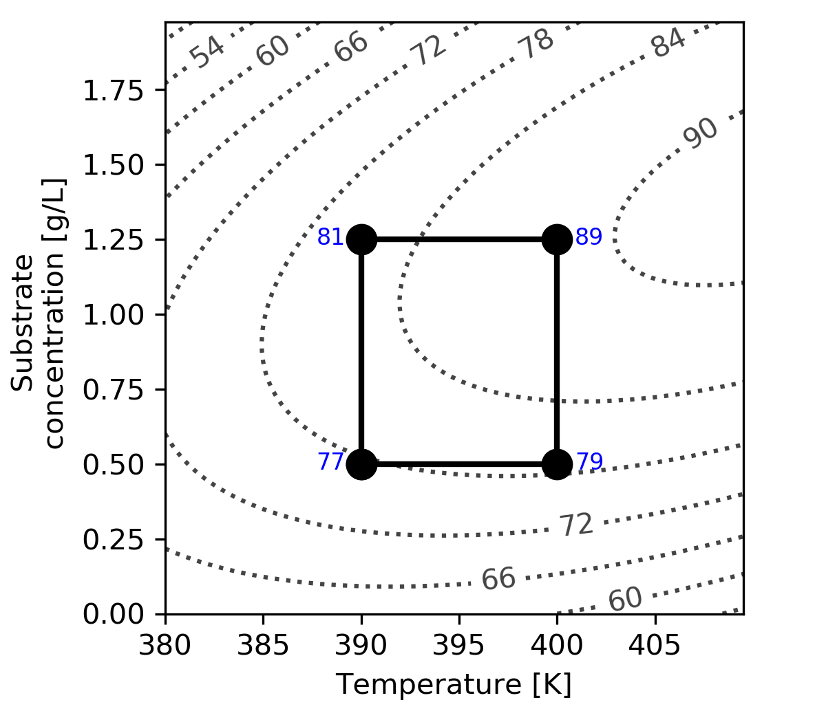
Let’s use a different system here to illustrate interaction effects, but still using \(T\) and \(S\) as the variables being changed and keeping the response variable, \(y\), as the conversion, shown by the contour lines.
Experiment
\(T\) [K]
\(S\) [g/L]
\(y\) [%]
1
\(-\) (390 K)
\(-\) (0.5 g/L)
77
2
\(+\) (400 K)
\(-\) (0.5 g/L)
79
3
\(-\) (390 K)
\(+\) (1.25 g/L)
81
4
\(+\) (400 K)
\(+\) (1.25 g/L)
89
The main effect of temperature for this system is
\(\Delta T_{S-} = 79 - 77 = 2\%\) per 10 K
\(\Delta T_{S+} = 89 - 81 = 8\%\) per 10 K
which means that the average temperature main effect is 5% per 10 K.
Notice how different the main effect is at the low and high levels of \(S\). So the average of the two is an incomplete description of the system. There is some other aspect to the system that we have not captured.
Similarly, the main effect of substrate concentration is
\(\Delta S_{T-} = 81 - 77 = 4\%\) per 0.75 g/L
\(\Delta S_{T-} = 89 - 79 = 10\%\) per 0.75 g/L
which gives the average substrate concentration main effect as 7% per 0.75 g/L.
The data may also be visualized using an interaction plot here, showing a higher degree of interaction.
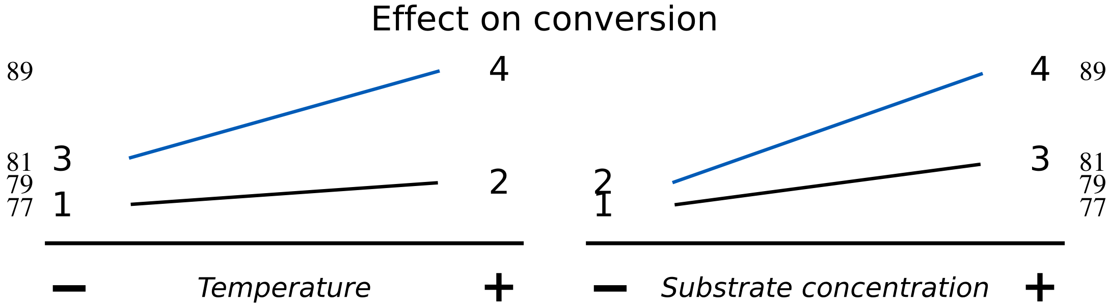
The lack of parallel lines is a clear indication of interaction. The temperature effect is stronger at high levels of \(S\), and the effect of \(S\) on conversion is also greater at high levels of temperature. What is missing is an interaction term, given by the product of temperature and substrate. We represent this as \(T \times S\) and call it the temperature-substrate interaction term.
This interaction term should be zero for systems with no interaction, which implies the lines are parallel in the interaction plot. Such systems will have roughly the same effect of \(T\) at both low and high values of \(S\) (and in between). So then, a good way to quantify interaction is by how different the main effect terms are at the high and low levels of the other factor in the interaction. The interaction must also be symmetrical: if \(T\) interacts with \(S\), then \(S\) interacts with \(T\) by the same amount.
We can quantify the interaction of our current example in this way. For the \(T\) interaction with \(S\):
Change in conversion due to \(T\) at high \(S\): \(89 - 81 = +8\)
Change in conversion due to \(T\) at low \(S\): \(79 - 77 = +2\)
The half difference: \([+8 - (+2)]/2 = \bf{3}\)
For the \(S\) interaction with \(T\),
Change in conversion due to \(S\) at high \(T\): \(89 - 79 = +10\)
Change in conversion due to \(S\) at low \(T\): \(81 - 77 = +4\)
The half difference: \([+10 - (+4)]/2 = \bf{3}\)
A large, positive interaction term indicates that temperature and substrate concentration will increase conversion by a greater amount when both \(T\) and \(S\) are high. Similarly, these two terms will rapidly reduce conversion when they both are low.
We will get an improved appreciation for interpreting main effects and the interaction effect when we consider the analysis in the form of a linear, least squares model.