2.5. Some terminology

We review a couple of concepts that you should have seen in a prior statistical course or elsewhere. If unfamiliar, please type the word or concept in a search engine for more background.

Population

A large collection of observations that might occur; a set of potential measurements. Some texts consider an infinite collection of observations, but a large number of observations is good enough.

Sample

A collection of observations that have actually occurred; a set of existing measurements that we have recorded in some way, usually electronically.

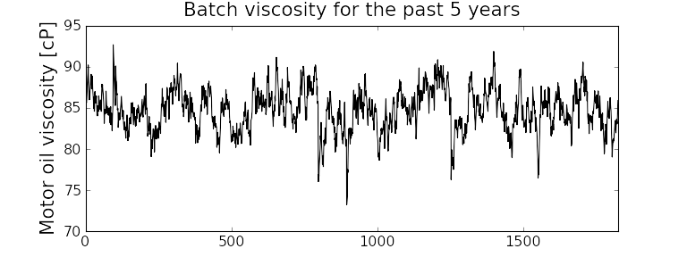
In engineering applications where we have plenty of data, we can characterize the population from all available data. The figure here shows the viscosity of a motor oil, from all batches produced in the last 5 years (about 1 batch per day). These 1825 data points, though technically a sample are an excellent surrogate for the population viscosity because they come from such a long duration. Once we have characterized these samples, future viscosity values will likely follow that same distribution, provided the process continues to operate in a similar manner.

Distribution

Distributions are used to summarize, in a compact way, a much larger collection of a much larger collection of data points. Histograms, just discussed above, are one way of visualizing a distribution. We can also express distributions by a few numerical parameters. See below.

Probability

The area under a plot of relative frequency distribution is equal to 1. Probability is then the fraction of the area under the frequency distribution curve (also called density curve).

Superimpose a vertical line on your fictitious histograms you drew earlier to indicate:

• the probability of a test grades less than 80%;

• the probability that the number thrown from a 6-sided die is less than or equal to 2;

• the probability of someone’s income exceeding $60000;

• the probability of the measurement exceeding a certain critical value.

Parameter

A parameter is a value that describes the population’s distribution in some way. For example, the population mean.

Statistic

A statistic is an estimate of a population parameter.

Mean (location)

The mean, or average, is a measure of location of the distribution. For each measurement, \(x_i\), in your sample

\begin{alignat*}{2} \text{population mean:} &\qquad& \mathcal{E}\left\{x \right\} = \mu &= \frac{1}{N}\sum{x} \\ \text{sample mean:} &\qquad& \overline{x} &= \frac{1}{n}\sum_{i=1}^{n}{x_i} \end{alignat*}

where \(N\) represents the size of the entire population, and \(n\) is the number of samples measured from the population.

This is only one of several statistics that describes your data: if you told your customer that the average density of your liquid product was 1.421 g/L, and nothing further, the customer might assume all lots of the same product have a density of 1.421 g/L. But we know from our earlier discussion that there will be variation. We need information, in addition to the mean, to quantify the distribution of values: the spread.

Variance (spread)

A measure of spread, or variance, is also essential to quantify your distribution.

\begin{alignat*}{2} \text{Population variance}: &\qquad& \mathcal{V}\left\{x\right\} = \mathcal{E}\left\{ (x - \mu )^2\right\} = \sigma^2 &= \frac{1}{N}\sum{(x-\mu)^2} \\ \text{Sample variance}: &\qquad& s^2 &= \frac{1}{n-1}\sum_{i=1}^{n}{(x_i - \overline{x})^2} \end{alignat*}

Dividing by \(n-1\) makes the variance statistic, \(s^2\), an unbiased estimator of the population variance, \(\sigma^2\). However, in many data sets our value for \(n\) is large, so using a divisor of \(n\), which you might come across in computer software or other texts, rather than \(n-1\) as shown here, leads to little difference.

The square root of variance, called the standard deviation is a more useful measure of spread: it is easier to visualize on a histogram and has the advantage of being in the same units of measurement as the variable itself.

Degrees of freedom

The denominator in the sample variance calculation, \(n-1\), is called the degrees of freedom. We have one fewer than \(n\) degrees of freedom, because there is a constraint that the sum of the deviations around \(\overline{x}\) must add up to zero. This constraint is from the definition of the mean. However, if we knew what the sample mean was without having to estimate it, then we could subtract each \(x_i\) from that value, and our degrees of freedom would be \(n\).

Outliers

Outliers are hard to define precisely, but an acceptable definition is that an outlier is a point that is unusual, given the context of the surrounding data. Another definition which is less useful, but nevertheless points out the problem of concretely defining what an outlier is, is this: “An outlier - I know it when I see it!”

The following 2 sequences of numbers show the number 4024 that appears in the first sequence, has become an outlier in the second sequence. It is an outlier based on the surrounding context.

• 4024, 5152, 2314, 6360, 4915, 9552, 2415, 6402, 6261

• 4, 61, 12, 64, 4024, 52, -8, 67, 104, 24

Median (robust measure of location)

The median is an alternative measure of location. It is a sample statistic, not a population statistic, and is computed by sorting the data and taking the middle value (or average of the middle 2 values, for even \(n\)). It is also called a robust statistic, because it is insensitive (robust) to outliers in the data.

Note

The median is the most robust estimator of the sample location: it has a breakdown of 50%, which means that just under 50% of the data need to be replaced with unusual values before the median breaks down as a suitable estimate. The mean on the other hand has a breakdown value of \(1/n\), as only one of the data points needs to be unusual to cause the mean to be a poor estimate. To compute the median in R, use the median(x) function on a vector x.

Governments will report the median income, rather than the mean, to avoid influencing the value with the few very high earners and the many low earners. The median income per person is a more fair measure of location in this case.

Median absolute deviation, MAD (robust measure of spread)

A robust measure of spread is the MAD, the median absolute deviation. The name is descriptive of how the MAD is computed:

\[\text{mad}\left\{ x_i \right\} = c \cdot \text{median}\left\{ \| x_i - \text{median}\left\{ x_i \right\} \| \right\} \qquad\qquad \text{where}\qquad c = 1.4826\]

The constant \(c\) makes the MAD consistent with the standard deviation when the observations \(x_i\) are normally distributed. The MAD has a breakdown point of 50%, because like the median, we can replace just under half the data with outliers before the MAD estimate becomes unbounded. To compute the MAD in R, use the mad(x) function on a vector x.

Enrichment reading: read pages 1 to 8 of “Tutorial to Robust Statistics”, PJ Rousseeuw, Journal of Chemometrics, 5, 1-20, 1991.