6.7.2. A conceptual explanation of PLS¶

Now that you are comfortable with the concept of a latent variable using PCA and PCR, you can interpret PLS as a latent variable model, but one that has a different objective function. In PCA the objective function was to calculate each latent variable so that it best explains the available variance in $\mathbf{X}_a$, where the subscript $A$ refers to the matrix $\mathbf{X}$ before extracting the $a^\text{th}$ component.

In PLS, we also find these latent variables, but we find them so they best explain $\mathbf{X}_a$ and best explain $\mathbf{Y}_a$, and so that these latent variables have the strongest possible relationship between $\mathbf{X}_a$ and $\mathbf{Y}_a$.

In other words, there are three simultaneous objectives with PLS:

The best explanation of the $\mathbf{X}$-space.

The best explanation of the $\mathbf{Y}$-space.

The greatest relationship between the $\mathbf{X}$- and $\mathbf{Y}$-space.

6.7.3. A mathematical/statistical interpretation of PLS¶

We will get back to the mathematical details later on, but we will consider our conceptual explanation above in terms of mathematical symbols.

In PCA, the objective was to best explain $\mathbf{X}_a$. To do this we calculated scores, $\mathbf{T}$, and loadings $\mathbf{P}$, so that each component, $\mathbf{t}_a$, had the greatest variance, while keeping the loading direction, $\mathbf{p}_a$, constrained to a unit vector.

\[\max : \mathbf{t}'_a \mathbf{t}_a \qquad \text{subject to}\quad \mathbf{p}'_a \mathbf{p}_a = 1.0\]

The above was shown to be a concise mathematical way to state that these scores and loadings best explain $\mathbf{X}$; no other loading direction will have greater variance of $\mathbf{t}'_a$. (The scores have mean of zero, so their variance is proportional to $\mathbf{t}'_a \mathbf{t}_a$).

For PCA, for the $a^\text{th}$ component, we can calculate the scores as follows (we are projecting the values in $\mathbf{X}_a$ onto the loading direction $\mathbf{p}_a$):

\[\mathbf{t}_a = \mathbf{X}_a \mathbf{p}_a\]

Now let’s look at PLS. Earlier we said that PLS extracts a single set of scores, $\mathbf{T}$, from $\mathbf{X}$ and $\mathbf{Y}$ simultaneously. That wasn’t quite true, but it is still an accurate statement! PLS actually extracts two sets of scores, one set for $\mathbf{X}$ and another set for $\mathbf{Y}$. We write these scores for each space as:

\begin{align*} \mathbf{t}_a &= \mathbf{X}_a \mathbf{w}_a \qquad &\text{for the $\mathbf{X}$-space} \\ \mathbf{u}_a &= \mathbf{Y}_a \mathbf{c}_a \qquad &\text{for the $\mathbf{Y}$-space} \end{align*}

The objective of PLS is to extract these scores so that they have maximal covariance. Let’s take a look at this. Covariance was shown to be:

\[\text{Cov}\left(\mathbf{t}_a, \mathbf{u}_a\right) = \mathcal{E}\left\{ (\mathbf{t}_a - \overline{\mathbf{t}}_a) (\mathbf{u}_a - \overline{\mathbf{u}}_a)\right\}\]

Using the fact that these scores have mean of zero, the covariance is proportional (with a constant scaling factor of $N$) to $\mathbf{t}'_a \mathbf{u}_a$. So in summary, each component in PLS is maximizing that covariance, or the dot product: $\mathbf{t}'_a \mathbf{u}_a$.

Now covariance is a hard number to interpret; about all we can say with a covariance number is that the larger it is, the greater the relationship, or correlation, between two vectors. So it is actually more informative to rewrite covariance in terms of correlations and variances:

\[\begin{split}\text{Cov}\left(\mathbf{t}_a, \mathbf{u}_a\right) &= \text{Correlation}\left(\mathbf{t}_a, \mathbf{u}_a\right) \times \sqrt{\text{Var}\left(\mathbf{t}_a\right)}\times \sqrt{\text{Var}\left(\mathbf{u}_a\right)} \\ \text{Cov}\left(\mathbf{t}_a, \mathbf{u}_a\right) &= \text{Correlation}\left(\mathbf{t}_a, \mathbf{u}_a\right) \times \sqrt{\mathbf{t}'_a \mathbf{t}_a} \times \sqrt{\mathbf{u}'_a \mathbf{u}_a} \\\end{split}\]

As this shows then, maximizing the covariance between $\mathbf{t}'_a$ and $\mathbf{u}_a$ is actually maximizing the 3 simultaneous objectives mentioned earlier:

The best explanation of the $\mathbf{X}$-space: given by $\mathbf{t}'_a \mathbf{t}_a$

The best explanation of the $\mathbf{Y}$-space. given by $\mathbf{u}'_a \mathbf{u}_a$

The greatest relationship between the $\mathbf{X}$- and $\mathbf{Y}$-space: given by $\text{correlation}\left(\mathbf{t}_a, \mathbf{u}_a\right)$

These scores, $\mathbf{t}'_a$ and $\mathbf{u}_a$, are found subject to the constraints that $\mathbf{\mathbf{w}'_a \mathbf{w}_a} = 1.0$ and $\mathbf{\mathbf{c}'_a \mathbf{c}_a} = 1.0$. This is similar to PCA, where the loadings $\mathbf{p}_a$ were constrained to unit length. In PLS we constrain the loadings for $\mathbf{X}$, called $\mathbf{w}_a$, and the loadings for $\mathbf{Y}$, called $\mathbf{c}_a$, to unit length.

The above is a description of one variant of PLS, known as SIMPLS (simple PLS).

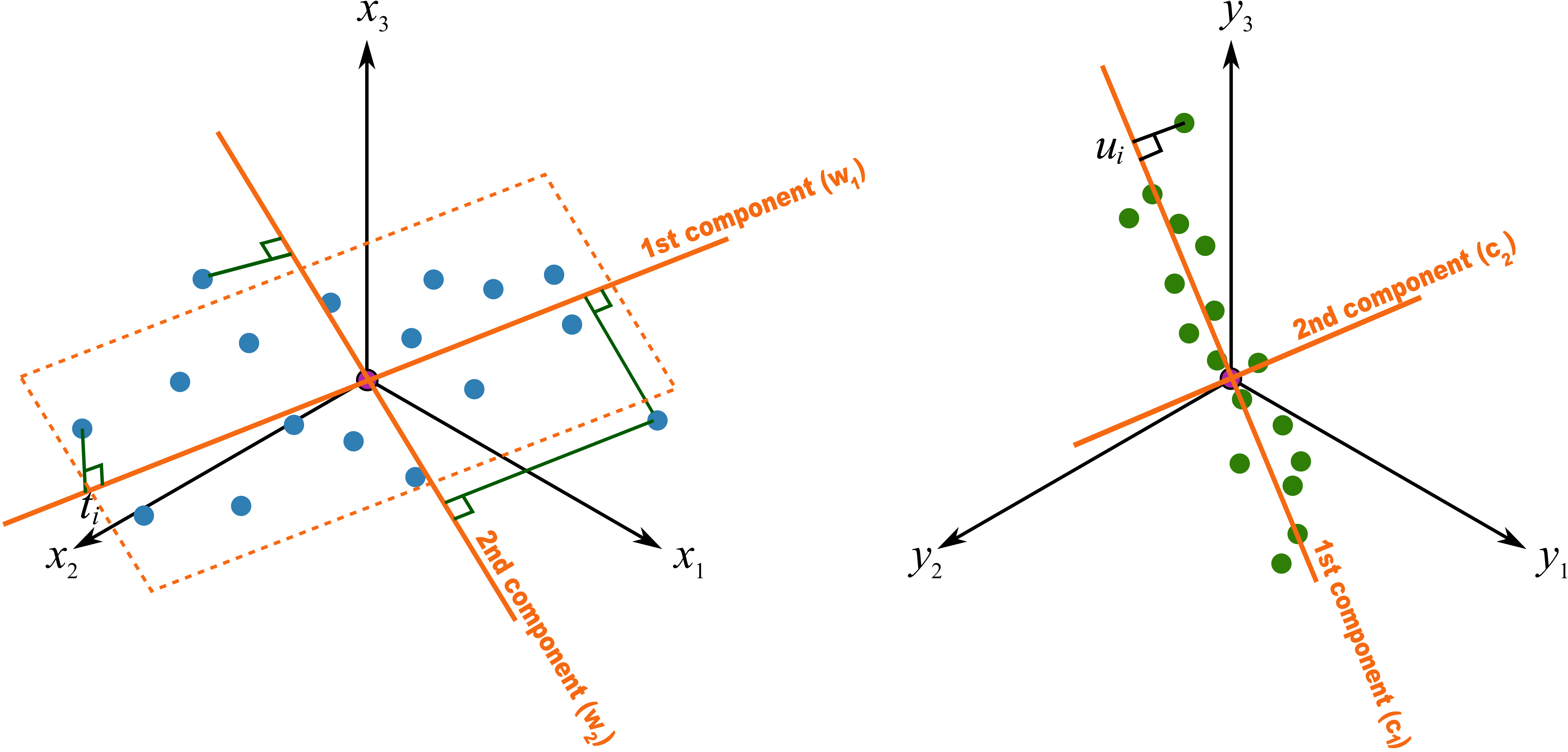
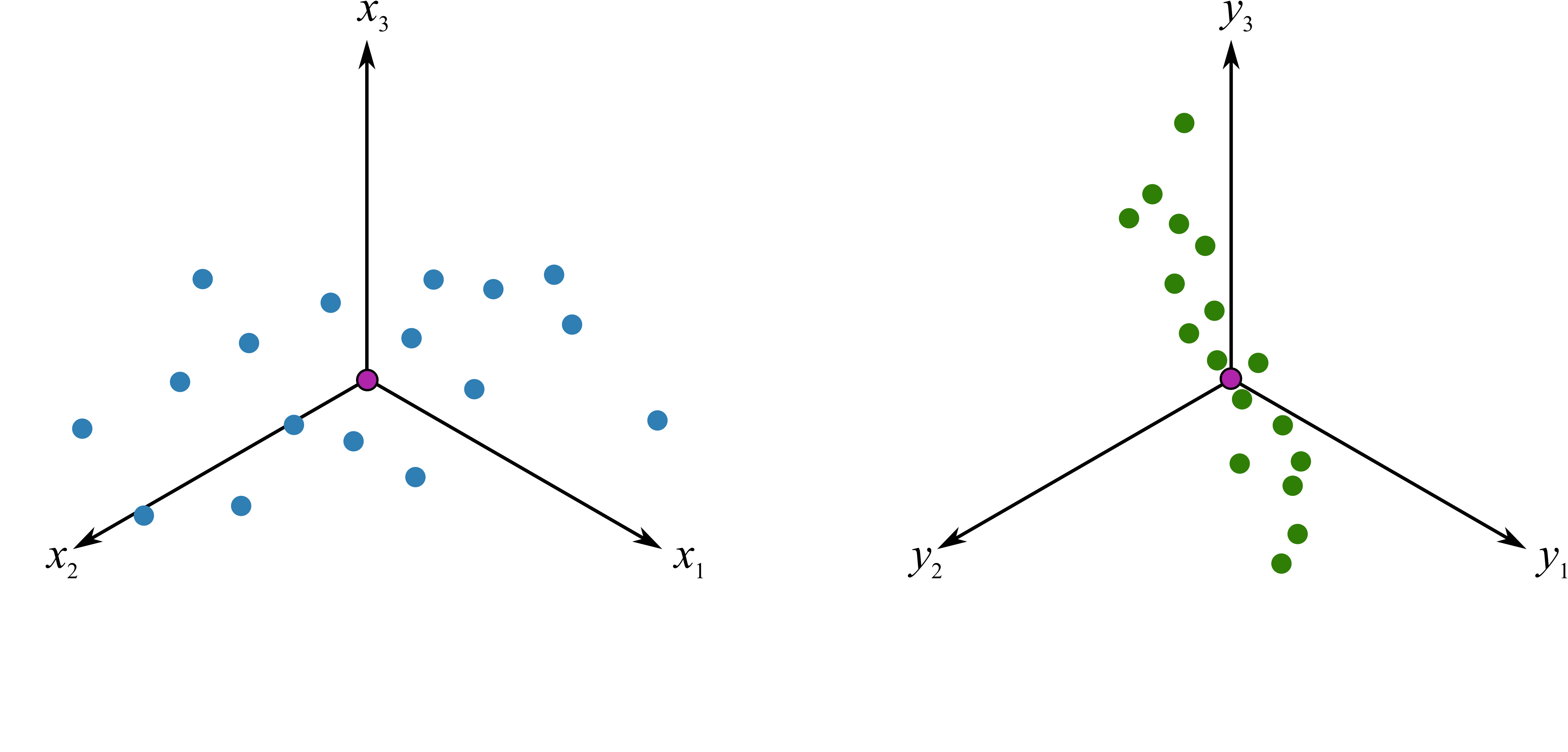
6.7.4. A geometric interpretation of PLS¶

As we did with PCA, let’s take a geometric look at the PLS model space. In the illustration below we happen to have $K=3$ variables in $\mathbf{X}$, and $M=3$ variables in $\mathbf{Y}$. (In general $K \neq M$, but $K=M=3$ make explanation in the figures easier.) Once the data are centered and scaled we have just shifted our coordinate system to the origin. Notice that there is one dot in $\mathbf{X}$ for each dot in $\mathbf{Y}$. Each dot represents a row from the corresponding $\mathbf{X}$ and $\mathbf{Y}$ matrix.

../../figures/pls/geometric-interpretation-of-PLS.svg

We assume here that you understand how the scores are the perpendicular projection of each data point onto each direction vector (if not, please review the relevant section in the PCA notes). In PLS though, the direction vectors, $\mathbf{w}_1$ and $\mathbf{c}_1$, are found and each observation is projected onto the direction. The point at which each observation lands is called the $\mathbf{X}$-space score, $t_i$, or the $\mathbf{Y}$-space score, $u_i$. These scores are found so that the covariance between the $t$-values and $u$-values is maximized.

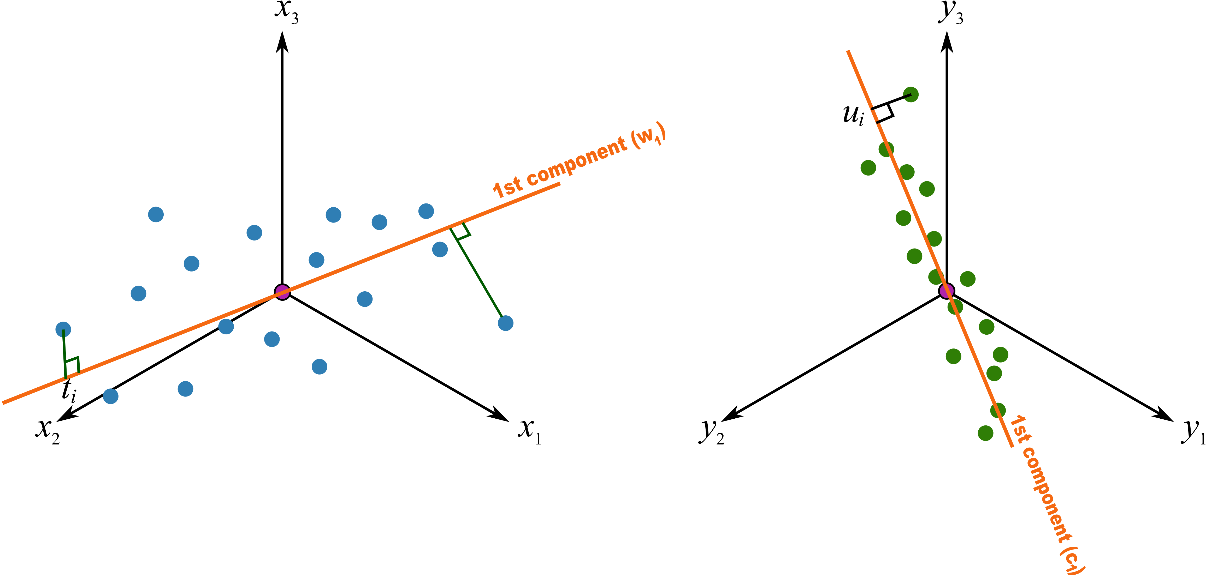
As explained above, this means that the latent variable directions are oriented so that they best explain $\mathbf{X}$, and best explain $\mathbf{Y}$, and have the greatest possible relationship between $\mathbf{X}$ and $\mathbf{Y}$.

The second component is then found so that it is orthogonal to the first component in the $\mathbf{X}$ space (the second component is not necessarily orthogonal in the $\mathbf{Y}$-space, though it often is close to orthogonal).