3.8. Process capability
Note
This section is not about a particular monitoring chart, but is relevant to the topic of process monitoring.
3.8.1. Centered processes
Purchasers of your product may request a process capability ratio (PCR) for each of the quality attributes of your product. For example, your plastic product is characterized by its Mooney viscosity and melting point. A PCR value can be calculated for either property, using the definition below:
Since the population standard deviation, \(\sigma\), is not known, an estimate of it is used. Note that the lower specification limit (LSL) and upper specification limit (USL) are not the same as the lower control limit (LCL) and upper control limit (UCL) as were calculated for the Shewhart chart. The LSL and USL are the tolerance limits required by your customers, or set from your internal specifications.
Interpretation of the PCR:
assumes the property of interest follows a normal distribution
assumes the process is centered (i.e. your long term mean is halfway between the upper and lower specification limits)
assumes the PCR value was calculated when the process was stable
The PCR is often called the process width. Let’s see why by taking a look at a process with PCR=0.5 and then PCR=2.0. In the first case \(\text{USL} - \text{LSL} = 3\sigma\). Since the interpretation of PCR assumes a centered process, we can draw a diagram as shown below:
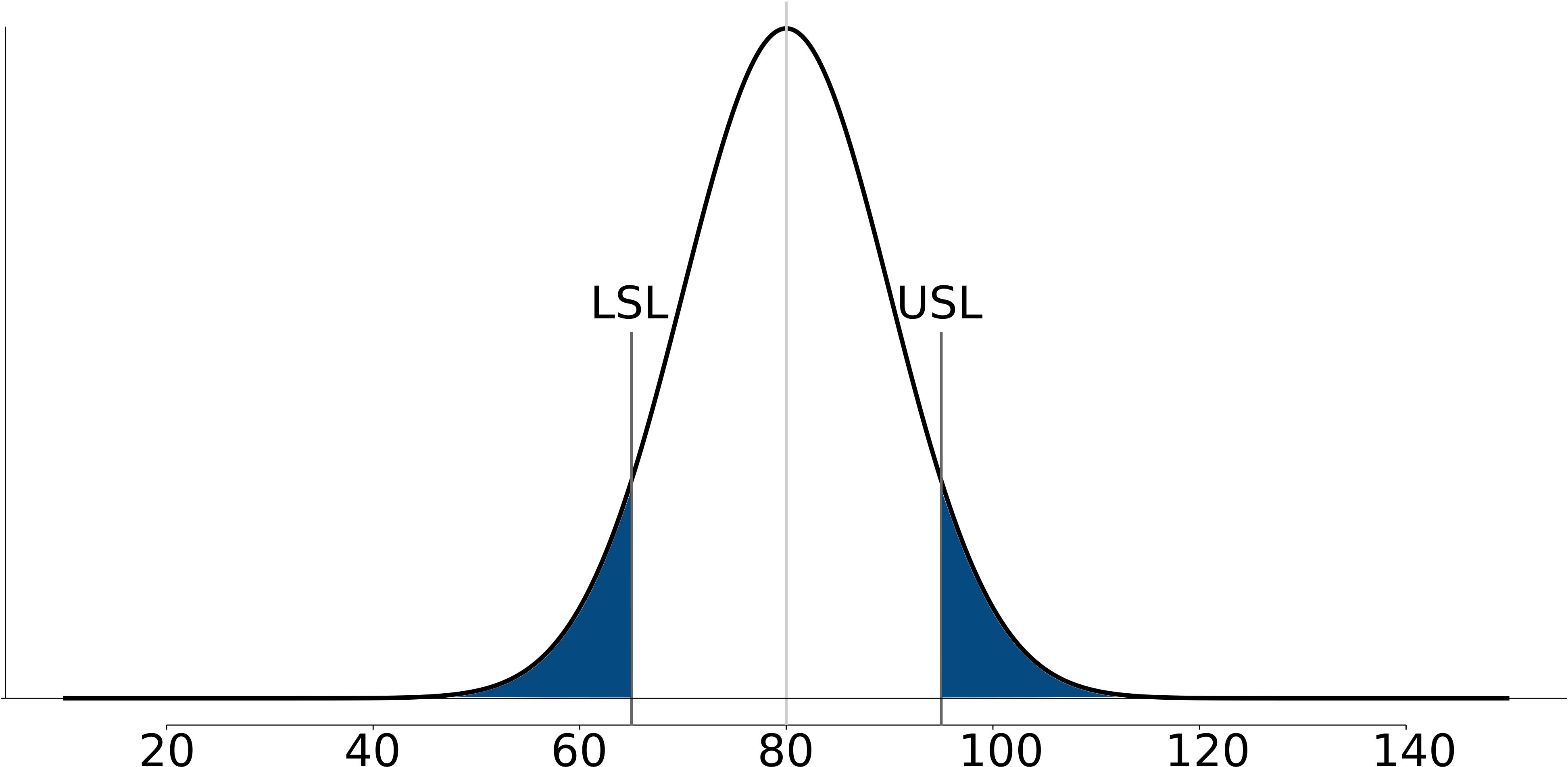
The diagram is from a process with mean of 80 and where LSL=65 and USL=95. These specification are fixed, set by our production guidelines. If the process variation is \(\sigma = 10\), then this implies that PCR=0.5. Assuming further that the our production is centered at the mean of 80, we can calculate how much defective product is produced in the shaded region of the plot. Assuming a normal distribution:
\(z\) for LSL = \((65 - 80)/10 = -1.5\)
\(z\) for USL = \((95 - 80)/10 = 1.5\)
Shaded area probability =
pnorm(-1.5) + (1-pnorm(1.5))= 13.4% of production is out of the specification limits.
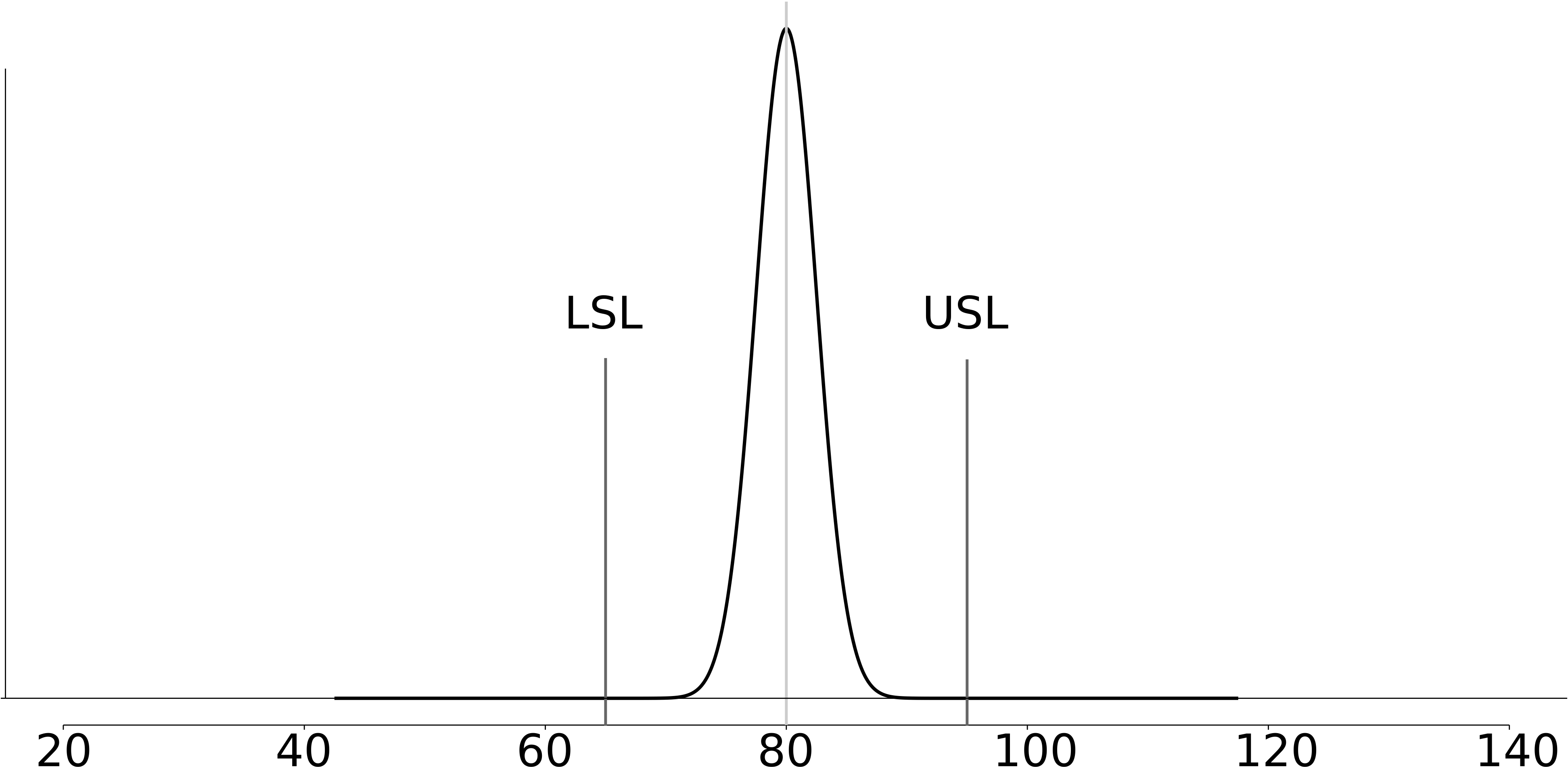
Contrast this to the case where PCR = 2.0 for the same system. To achieve that level of process capability, using the same upper and lower specifications we have to reduce the standard deviation by a factor of 4, down to \(\sigma = 2.5\). The figure below illustrates that almost no off-specification product is produced for a centered process at PCR = 2.0. There is a width of \(12 \sigma\) units from the LSL to the USL, giving the process location (mean) ample room to drift left or right without creating additional off-specification product.
Note
You will probably come across the terminology Cp, especially when dealing with 6 sigma programs. This is the same as PCR for a centered process.
3.8.2. Uncentered processes
Processes are not very often centered between their upper and lower specification limits. So a measure of process capability for an uncentered processes is defined:
The \(\overline{\overline{x}}\) term would be the process target from a Shewhart chart, or simply the actual average operating point. Notice that Cpk is a one-sided ratio, only the side closest to the specification is reported. So even an excellent process with Cp = 2.0 that is running off-center will have a lower Cpk.
It is the Cpk value that is requested by your customer. Values of 1.3 are usually a minimum requirement, while 1.67 and higher are requested for health and safety-critical applications. A value of Cpk \(\geq 2.0\) is termed a six-sigma process, because the distance from the current operating point, \(\overline{\overline{x}}\), to the closest specification is at least \(6\sigma\) units.
You can calculate that a shift of \(1.5\sigma\) from process center will introduce only 3.4 defects per million. This shift would reduce your Cpk from 2.0 to 1.5.
Note
It must be emphasized that Cpk and Cp numbers are only useful for a process which is stable. Furthermore the assumption of normally distributed samples is also required to interpret the Cpk value.