4.8. Investigating an existing linear model¶

4.8.1. Summary so far¶

We have introduced the linear model, $y = \beta_0 + \beta_1 x + \varepsilon$ and shown how to estimate the 2 model parameters, $b_0 = \hat{\beta}_0$ and $b_1 = \hat{\beta}_1$. This can be done on any data set without any additional assumptions. But, in order to calculate confidence intervals so we can better understand our model’s performance, we must make several assumptions of the data. In the next sections we will learn how to interpret various plots that indicate when these assumptions are violated.

Along the way, while investigating these assumptions, we will introduce some new topics:

Transformations of the raw data to better meet our assumptions

Leverage, outliers, influence and discrepancy of the observations

Inclusion of additional terms in the linear model (multiple linear regression, MLR)

The use of training and testing data

It is a common theme in any modelling work that the most informative plots are those of the residuals - the unmodelled component of our data. We expect to see no structure in the residuals, and since the human eye is excellent at spotting patterns in plots, it is no surprise that various types of residual plots are used to diagnose problems with our model.

4.8.2. The assumption of normally distributed errors¶

We look for normally distributed errors because if they are non-normal, then the standard error, $S_E$ and the other variances that depend on $S_E$, such as $\mathcal{V}(b_1)$, could be inflated, and their interpretation could be in doubt. This might, for example, lead us to infer that a slope coefficient is not important when it actually is.

This is one of the easiest assumptions to verify: use a q-q plot to assess the distribution of the residuals. Do not plot the residuals in sequence or some other order to verify normality - it is extremely difficult to see that. A q-q plot highlights very clearly when tails from the residuals are too heavy. A histogram may also be used, but for real data sets, the choice of bin width can dramatically distort the interpretation - rather use a q-q plot. Some code for R:

model = lm(...)
library(car)
qqPlot(model)            # uses studentized residuals
qqPlot(resid(model))     # uses raw residuals

If the residuals appear non-normal, then attempt the following:

Remove the outlying observation(s) in the tails, but only after careful investigation whether that outlier really was unusual

Use a suitable transformation of the y-variable

Add additional terms to the least squares model

The simple example shown here builds a model that predicts the price of a used vehicle using only the mileage as an explanatory variable.

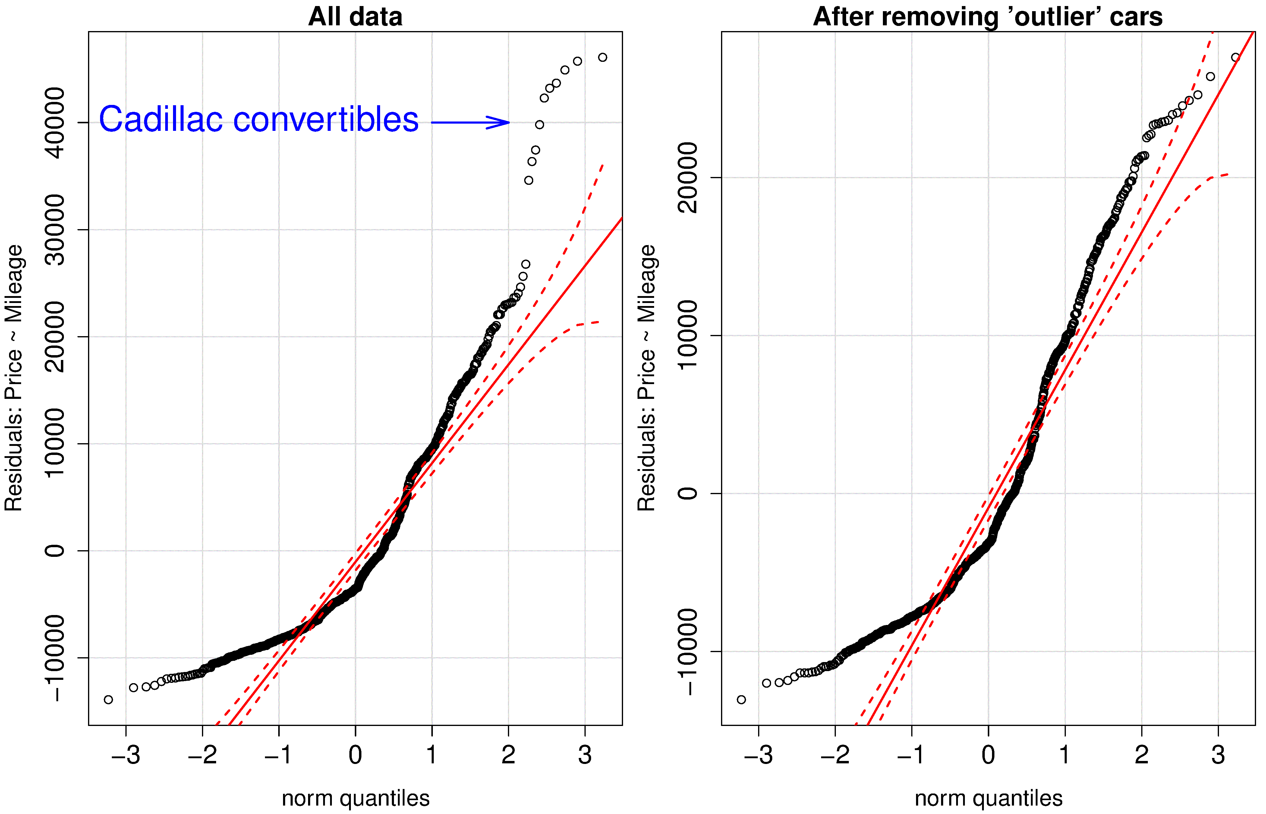
The group of outliers were due to 10 observations of a certain class of vehicle (Cadillac convertibles) that distorted the model. We removed these observations, which now limits our model to be useful only for other vehicle types, but we gain a smaller standard error and a tighter confidence interval. These residuals are still very non-normal though.

\[\begin{split}\begin{array}{rcccl} \text{Before}: \qquad & b_1 = -0.173 & \qquad -0.255 \leq \beta_1 \leq -0.0898 &\qquad S_E = \text{\$} 9789\\ \text{After}: \qquad & b_1 = -0.155 & \qquad -0.230 \leq \beta_1 \leq -0.0807 &\qquad S_E = \text{\$} 8655 \end{array}\end{split}\]

The slope coefficient (interpretation: each extra mile on the odometer reduces the sale price on average by 15 to 17 cents) has a tighter confidence interval after removing those unusual observations.

Removing the Cadillac cars from our model indicates that there is more than just mileage that affect their resale value. In fact, the lack of normality, and structure in the residuals leads us to ask which other explanatory variables can be included in the model.

In the next fictitious example the $\mathrm{y}$-variable is non-linearly related to the $\mathrm{x}$-variable. This non-linearity in the $\mathrm{y}$ shows up as non-normality in the residuals if only a linear model is used. The residuals become more linearly distributed when using a square root transformation of the $\mathrm{y}$ before building the linear model.

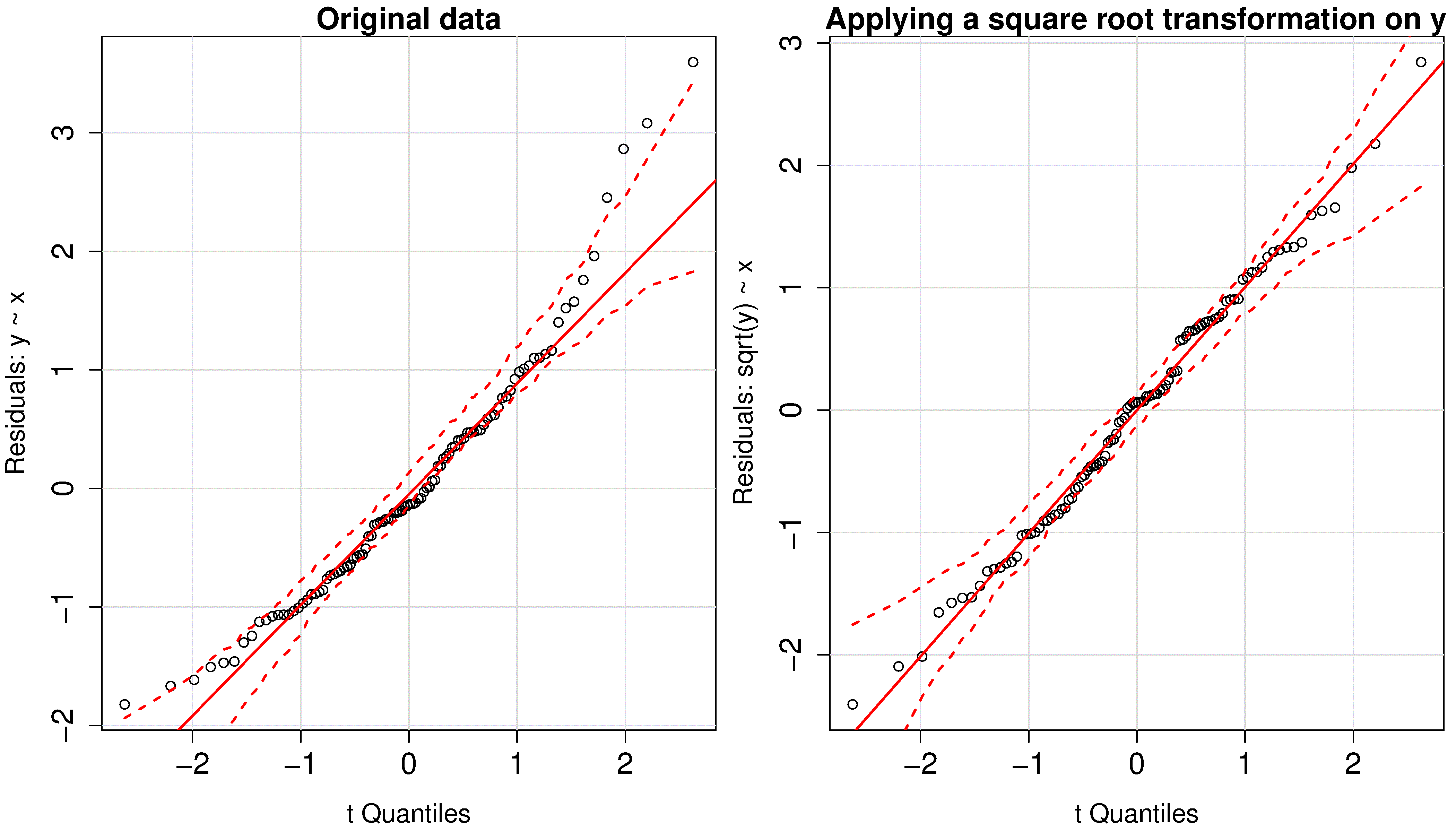
More discussion about transformations of the data is given in the section on model linearity.

4.8.3. Non-constant error variance¶

It is common in many situations that the variability in $\mathrm{y}$ increases or decreases as $\mathrm{y}$ is increased (e.g. certain properties are more consistently measured at low levels than at high levels). Similarly, variability in $\mathrm{y}$ increases or decreases as $\mathrm{x}$ is increased (e.g. as temperature, $\mathrm{x}$, increases the variability of a particular $\mathrm{y}$ increases).

Violating the assumption of non-constant error variance increases the standard error, $S_E$, undermining the estimates of the confidence intervals, and other analyses that depend on the standard error. Fortunately, it is only problematic if the non-constant variance is extreme, so we can tolerate minor violations of this assumption.

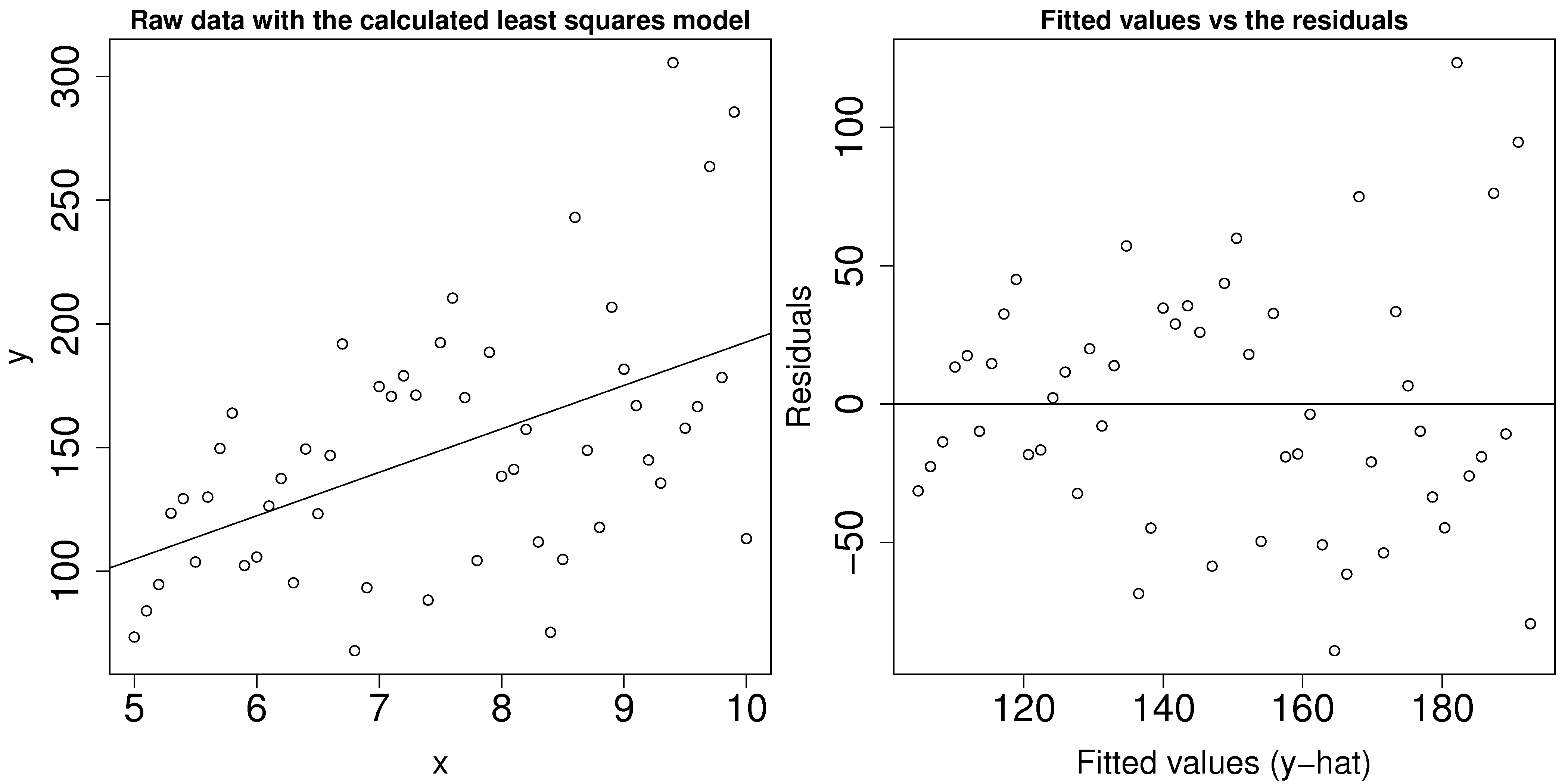
To detect this problem you should plot:

the predicted values of $\mathrm{y}$ (on the x-axis) against the residuals (y-axis)

the $\mathrm{x}$ values against the residuals (y-axis)

This problem reveals itself by showing a fan shape across the plot; an example is shown in the figure.

To counteract this problem one can use weighted least squares, with smaller weights on the high-variance observations, i.e. apply a weight inversely proportional to the variance. Weighted least squares minimizes: $f(\mathrm{b}) = \sum_i^n{(w_ie_i)^2}$, with different weights, $w_i$ for each error term. More on this topic can be found in the book by Draper and Smith (p 224 to 229, 3rd edition).

4.8.4. Lack of independence in the data¶

The assumption of independence in the data requires that values in the $\mathrm{y}$ variable are independent. Given that we have assumed the $\mathrm{x}$ variable to be fixed, this implies that the errors, $e_i$ are independent. The reason for independence is required for the central limit theorem, which was used to derive the various standard errors.

Data are not independent when they are correlated with each other. This is common on slow moving processes: for example, measurements taken from a large reactor are unlikely to change much from one minute to the next.

Treating this problem properly comes under the topic of time-series analysis, for which a number of excellent textbooks exist, in particular the one by Box and Jenkins. But we will show how to detect autocorrelation, and provide a make-shift solution to avoid it.

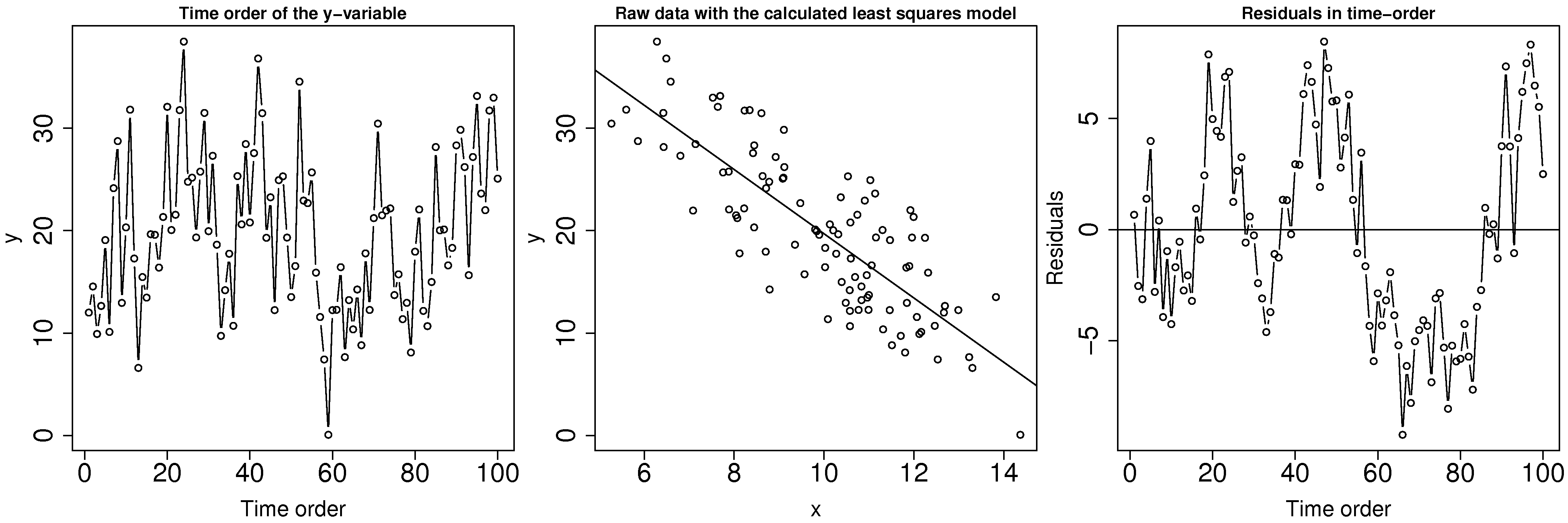
If you suspect that there may be lack of independence, use plots of the residuals in time order. Look for patterns such as slow drifts, or rapid criss-crossing of the zero axis.

One way around the autocorrelation is to subsample - use only every $k^\text{th}$ sample, where $k$ is a certain number of gaps between the points. How do we know how many gaps to leave? Use the autocorrelation function to determine how many samples. You can use the acf(...) function in R, which will show how many significant lags there are between observations. Calculating the autocorrelation accurately requires a large data set, which is a requirement anyway if you need to subsample your data to obtain independence.

Here are some examples of the autocorrelation plot: in the first case you would have to leave at least 16 samples between each sub-sample, while the second and third cases require a gap of 1 sample, i.e. use only every second data point.

Another test for autocorrelation is the Durbin-Watson test. For more on this test see the book by Draper and Smith (Chapter 7, 3rd edition); in R you can use the durbinWatsonTest(model) function in library(car). Try generating autocorrelation of varying strength (positive, e.g. phi_long = 0.80 and negative, e.g. phi_long = -0.75) in the code below. Inspect the plots which are generated as a result, especially the time order plot: get a feeling for what a strong and weak positive/negative correlation looks like in the time order.

4.8.5. Linearity of the model (incorrect model specification)¶

Recall that the linear model is just a tool to either learn more about our data, or to make predictions. Many cases of practical interest are from systems where the general theory is either unknown, or too complex, or known to be non-linear.

Certain cases of non-linearity can be dealt with by simple transformations of the raw data: use a non-linear transformation of the raw data and then build a linear model as usual. An alternative method which fits the non-linear function, using concepts of optimization, by minimizing the sum of squares is covered in a section on non-linear regression. Again the book by Draper and Smith (Chapter 24, 3rd edition), may be consulted if this topic is of further interest to you. Let’s take a look at a few examples.

We saw earlier a case where a square-root transformation of the $\mathrm{y}$ variable made the residuals more normally distributed. There is in fact a sequence of transformations that can be tried to modify the distribution of a single variable: $x_\text{transformed} \leftarrow x^p_\text{original}$.

When $p$ goes from 1 and higher, say 1.5, 1.75, 2.0, etc, it compresses small values of $x$ and inflates larger values.

When $p$ goes down from 1, 0.5 ($\sqrt{x}$), 0.25, -0.5, -1.0 ($1/x$), -1.5, -2.0, etc, it compresses large values of $x$ and inflates smaller values.

The case of $\log(x)$ approximates $p=0$ in terms of the severity of the transformation.

In other instances we may know from first-principles theory, or some other means, what the expected non-linear relationship is between an $\mathrm{x}$ and $\mathrm{y}$ variable.

In a distillation column the temperature, $T$ is inversely proportional to the logarithm of the vapour pressure, $P$. So fit a linear model, $y = b_0 + b_1x$ where $x \leftarrow 1/T$ and where $y \leftarrow P$. The slope coefficient will have a different interpretation and a different set of units as compared to the case when predicting vapour pressure directly from temperature.

If $y = p \times q^x$, then we can take logs and estimate this equivalent linear model: $\log(y) = \log(p) + x \log(q)$, which is of the form $y = b_0 + b_1 x$. So the slope coefficient will be an estimate of $\log(q)$.

If $y = \dfrac{1}{p+qx}$, then invert both sides and estimate the model $y = b_0 + b_1 x$ where $b_0 \leftarrow p$, $b_1 \leftarrow q$ and $y\leftarrow 1/y$.

There are plenty of other examples, some classic cases being the non-linear models that arise during reactor design and biological growth rate models. With some ingenuity (taking logs, inverting the equation), these can often be simplified into linear models.

Some cases cannot be linearized and are best estimated by non-linear least squares methods. However, a make-shift approach which works quite well for simple cases is to perform a grid search. For example imagine the equation to fit is $y = \beta_1\left(1-e^{-\beta_2 x} \right)$, and you are given some data pairs $(x_i, y_i)$. Then for example, create a set of trial values $\beta_1 = [10, 20, 30, 40, 50]$ and $\beta_2 = [0.0, 0.2, 0.4, 0.8]$. Build up a grid for each combination of $\beta_1$ and $\beta_2$ and calculate the sum of squares objective function for each point in the grid. By trial-and-error you can converge to an approximate value of $\beta_1$ and $\beta_2$ that best fit the data. You can then calculate $S_E$, but not the confidence intervals for $\beta_1$ and $\beta_2$.

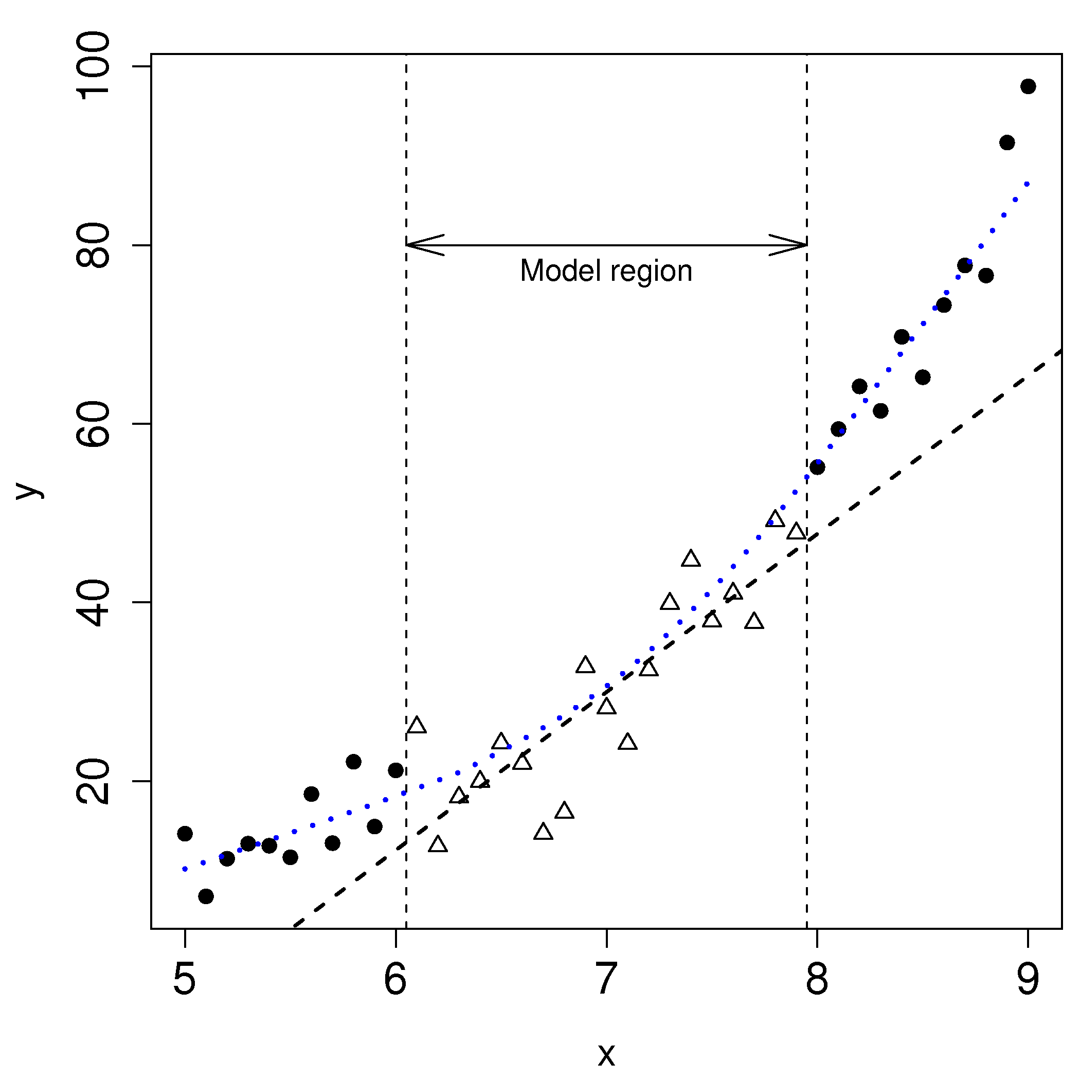
Before launching into various transformations or non-linear least squares models, bear in mind that the linear model may be useful over the region of interest. In the figure we might only be concerned with using the model over the region shown, even though the system under observation is known to behave non-linearly over a wider region of operation.

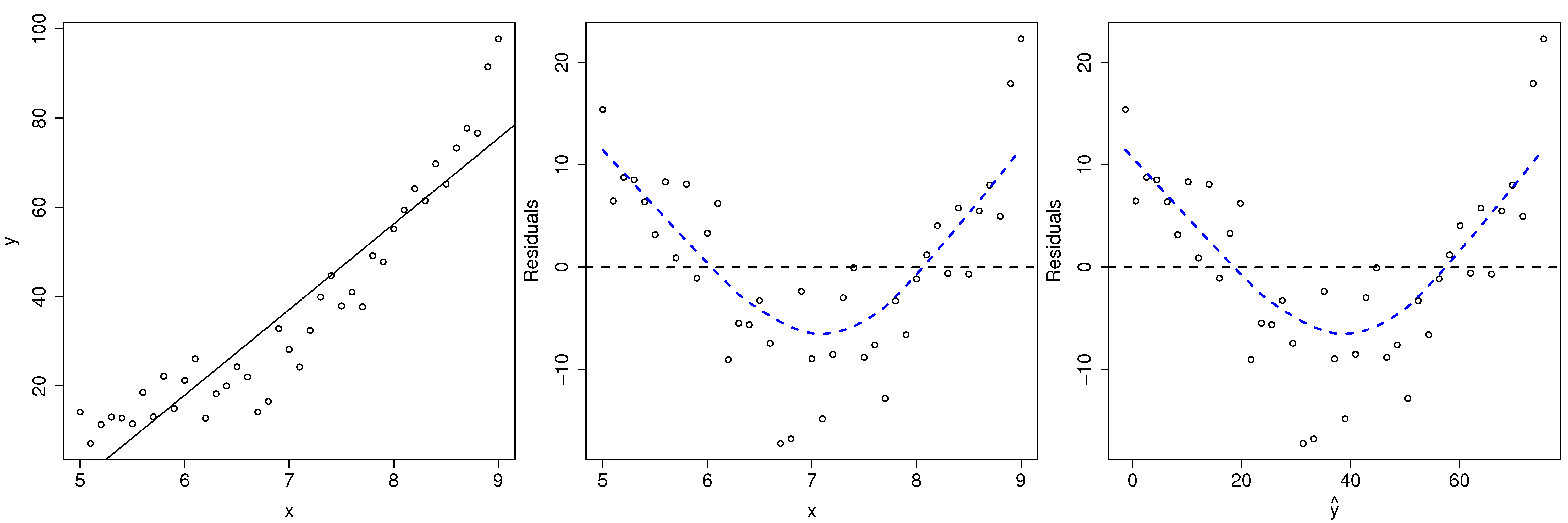
How can we detect when the linear model is not sufficient anymore? While a q-q plot might hint at problems, better plots are the same two plots for detecting non-constant error variance:

the predicted values of $\mathrm{y}$ (on the x-axis) against the residuals (y-axis)

the $\mathrm{x}$ values against the residuals (y-axis)

Here we show both plots for the example just prior (where we used a linear model for a smaller sub-region). The last two plots look the same, because the predicted $\hat{\mathrm{y}}$ values, $\hat{\mathrm{y}} = b_0 + b_1 x_1$; in other words, just a linear transformation of the $\mathrm{x}$ values.

Transformations are considered successful once the residuals appear to have no more structure in them. Also bear in mind that structure in the residuals might indicate the model is missing an additional explanatory variable (see the section on multiple linear regression).

Another type of plot to diagnose non-linearity present in the linear model is called a component-plus-residual plot or a partial-residual plot. This is an advanced topic not covered here, but well covered in the Fox reference.