6.7.11. PLS Exercises

6.7.11.1. The taste of cheddar cheese

• \(N=30\)

• \(K=3\)

• \(M=1\)

• Link to cheese data

• Description: This very simple case study considers the taste of mature cheddar cheese. There are 3 measurements taken on each cheese: lactic acid, acetic acid and \(\text{H}_2\text{S}\).

1. Import the data into R: cheese <- read.csv('http://openmv.net/file/cheddar-cheese.csv')

2. Use the car library and plot a scatter plot matrix of the raw data:

   • library(car)

   • scatterplotMatrix(cheese[,2:5])

   

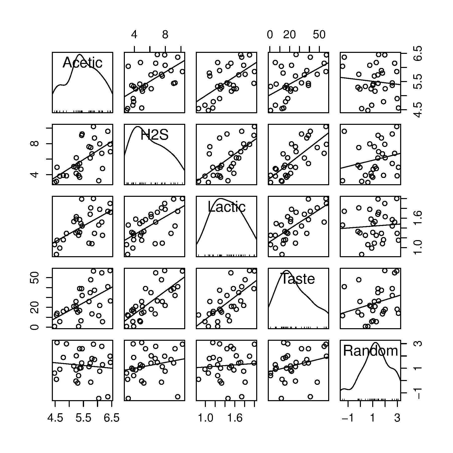
3. Using this figure, how many components do you expect to have in a PCA model on the 3 \(\mathbf{X}\) variables: Acetic, H2S and Lactic?

4. What would the loadings look like?

5. Build a PCA model now to verify your answers.

6. Before building the PLS model, how many components would you expect? And what would the weights look like (\(\mathbf{r}_1\), and \(\mathbf{c}_1\))?

7. Build a PLS model and plot the \(\mathbf{r:c}_1\) bar plot. Interpret it.

8. Now plot the SPE plot; these are the SPE values for the projections onto the \(\mathbf{X}\)-space. Any outliers apparent?

9. In R, build a least squares model that regresses the Taste variable on to the other 3 \(\mathbf{X}\) variables.

   • model.lm <- lm(Taste ~ Acetic + H2S + Lactic, data=cheese)

   • Report each coefficient \(\pm 2 S_E(b_i)\). Which coefficients does R find significant in MLR? (You can use the confint(model.lm) function too.)

     \[\begin{split}\beta_\text{Acetic} &= \qquad \qquad \pm \\ \beta_\text{H2S} &= \qquad \qquad \pm \\ \beta_\text{Lactic} &= \qquad \qquad \pm\end{split}\]

   • Report the standard error and the \(R^2_y\) value for this model.

   • Compare this to the PLS model’s \(R^2_y\) value.

10. Now build a PCR model in R using only 1 component, then using 2 components. Again calculate the standard error and \(R^2_y\) values.

11. Plot the observed \(\mathrm{y}\) values against the predicted \(\mathrm{y}\) values for the PLS model.

12. PLS models do not have a standard error, since the degrees of freedom are not as easily defined. But you can calculate the RMSEE (root mean square error of estimation) = \(\sqrt{\dfrac{\mathbf{e}'\mathbf{e}}{N}}\). Compare the RMSEE values for all the models just built.

Obviously the best way to test the model is to retain a certain amount of testing data (e.g. 10 observations), then calculate the root mean square error of prediction (RMSEP) on those testing data.

6.7.11.2. Comparing the loadings from a PCA model to a PLS model

PLS explains both the \(\mathbf{X}\) and \(\mathbf{Y}\) spaces, as well as building a predictive model between the two spaces. In this question we explore two models: a PCA model and a PLS model on the same data set.

The data are from the plastic pellets troubleshooting example.

• \(N = 24\)

• \(K = 6 + 1\) designation of process outcome

• Link to raw materials data

• Description: 3 of the 6 measurements are size values for the plastic pellets, while the other 3 are the outputs from thermogravimetric analysis (TGA), differential scanning calorimetry (DSC) and thermomechanical analysis (TMA), measured in a laboratory. These 6 measurements are thought to adequately characterize the raw material. Also provided is a designation Adequate or Poor that reflects the process engineer’s opinion of the yield from that lot of materials.

1. Build a PCA model on all seven variables, including the 0-1 process outcome variable in the \(\mathbf{X}\) space. Previously we omitted that variable from the model, this time include it.

2. How do the loadings look for the first, second and third components?

3. Now build a PLS model, where the \(\mathbf{Y}\)-variable is the 0-1 process outcome variable. In the previous PCA model the loadings were oriented in the directions of greatest variance. For the PLS model the loadings must be oriented so that they also explain the \(\mathbf{Y}\) variable and the relationship between \(\mathbf{X}\) and \(\mathbf{Y}\). Interpret the PLS loadings in light of this fact.

4. How many components were required by cross-validation for the PLS model?

5. Explain why the PLS loadings are different to the PCA loadings.

6.7.11.3. Predicting final quality from on-line process data: LDPE system

• \(N = 54\)

• \(K = 14\)

• \(K = 5\)

• Link to dataset website and description of the data.

1. Build a PCA model on the 14 \(\mathbf{X}\)-variables and the first 50 observations.

2. Build a PCA model on the 5 \(\mathbf{Y}\)-variables: Conv, Mn, Mw, LCB, and SCB. Use only the first 50 observations

3. Build a PLS model relating the \(\mathbf{X}\) variables to the \(\mathbf{Y}\) variables (using \(N=50\)). How many components are required for each of these 3 models?

4. Compare the loadings plot from PCA on the \(\mathbf{Y}\) space to the weights plot (\(\mathbf{c}_1\) vs \(\mathbf{c}_2\)) from the PLS model.

5. What is the \(R^2_X\) (not for \(\mathbf{Y}\)) for the first few components?

6. Now let’s look at the interpretation between the \(\mathbf{X}\) and \(\mathbf{Y}\) space. Which plot would you use?

   • Which variable(s) in \(\mathbf{X}\) are strongly related to the conversion of the product (Conv)? In other words, as an engineer, which of the 14 \(\mathbf{X}\) variables would you consider adjusting to improve conversion.

   • Would these adjustments affect any other quality variables? How would they affect the other quality variables?

   • How would you adjust the quality variable called Mw (the weight average molecular weight)?