5.14. Extended topics related to designed experiments

This section is just an overview of some interesting topics, together with references to guide you to more information.

5.14.1. Experiments with mistakes, missing values, or belatedly discovered constraints

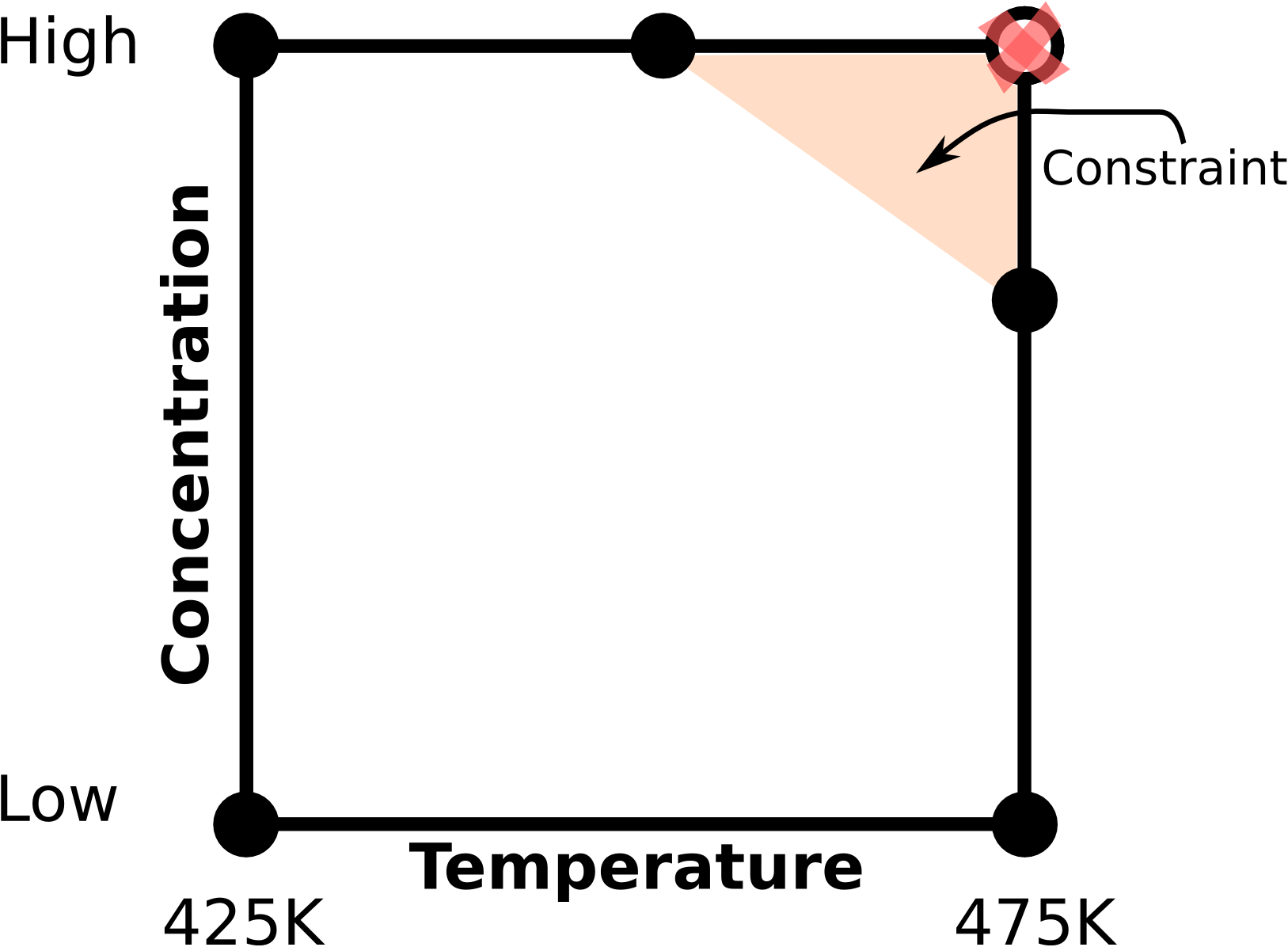
Many real experiments do not go smoothly. Once the experimenter has established their \(-1\) and \(+1\) levels for each variable, they back that out to real units. For example, if temperature was scaled as \(T = \dfrac{T_\text{actual} - 450\text{K}}{\text{25K}}\), then \(T = -1\) corresponds to 425K and \(T= +1\) corresponds to 475K.

But if the operator mistakenly sets the temperature to \(T_\text{actual} = 465K\), then it doesn’t quite reach the +1 level required. This is not a wasted experiment. Simply code this as \(T = \dfrac{465 - 450}{25} = 0.6\), and enter that value in the least squares model for matrix \(\mathbf{X}\). Then proceed to calculate the model parameters using the standard least squares equations. Note that the columns in the X-matrix will not be orthogonal anymore, so \(\mathbf{X}^T\mathbf{X}\) will not be a diagonal matrix, but it will be almost diagonal.

Similarly, it might be discovered that temperature cannot be set to 475K when the other factor, for example concentration, is also at its high level. This might be due to physical or safety constraints. On the other hand, \(T=475K\) can be used when concentration is at its low level. This case is the same as described above: set the temperature to the closest possible value for that experiment, and then analyze the data using a least squares model. The case when the constraint is known ahead of time is dealt with later on, but in this case, the constraint was discovered just as the run was to be performed.

Also see the section on optimal designs for how one can add one or more additional experiments to fix an existing bad set of experiments.

The other case that happens occasionally is that samples are lost, or the final response value is missing for some reason. Not everything is lost: recall the main effects for a full \(2^k\) factorial are estimated \(k\) times at each combination of the factors.

If one or more experiments have missing \(y\) values, you can still estimate these main effects, and sometimes the interaction parameters by hand. Furthermore, analyzing the data in a least squares model will be an undetermined system: more unknowns than equations. You could choose to drop out higher-order interaction terms to reduce the equations to a square system: as many unknowns as equations. Then proceed to analyze the results from the least squares model as usual. There are actually slightly more sophisticated ways of dealing with this problem, as described by Norman Draper in “Missing Values in Response Surface Designs”, Technometrics, 3, 389-398, 1961.

The above discussion illustrates clearly our preference for using the least squares model: whether the experimental design was executed accurately or not: the least squares model always works, whereas the short cut tools developed for perfectly executed experiments will fail.

5.14.2. Handling of constraints

Most engineering systems have limits of performance, either by design or from a safety standpoint. It is also common that optimum production levels are found close to these constraints. The factorials we use in our experiments must, by necessity, span a wide range of operation so that we see systematic change in our response variables, and not merely measure noise. These large ranges that we choose for the factors often hit up again constraints.

A simple bioreactor example for 2 factors is shown: at high temperatures and high substrate concentrations we risk activating a different, undesirable side-reaction. The shaded region represents the constraint where we may not operate. We could for example replace the \((T_{+}, C_{+})\) experiment with two others, and then analyze these 5 runs using least squares.

Unfortunately, these 5 runs do not form an orthogonal (independent) \(\mathbf{X}\) matrix anymore. We have lost orthogonality. We have also reduced the space (or volume when we have 3 or more factors) spanned by the factorial design.

It is easy to find experiments that obey the constraints for 2-factor cases: run them on the corner points. But for 3 or more factors the constraints form planes that cut through a cube. We then use optimal designs to determine where to place our experiments. A D-optimal design works well for constraint-handling because it finds the experimental points that would minimize the loss of orthogonality (i.e. they try to achieve the most orthogonal design possible). A compact way of stating this is to maximize the determinant of \(\mathbf{X}^T\mathbf{X}\), which is why it is called D-optimal (it maximizes the determinant).

These designs are generated by a computer, using iterative algorithms. See the D-optimal reference in the section on optimal designs for more information.

5.14.3. Optimal designs

If you delve into the modern literature on experimental methods you will rapidly come across the concept of an optimal design. This begs the question, what is sub-optimal about the factorial designs we have focussed on so far?

A full factorial design spans the maximal space possible for the \(k\) factors. From least squares modelling we know that large deviations from the model center reduces the variance of the parameter estimates. Furthermore, a factorial ensures the factors are moved independently, allowing us to estimate their effects independently as well. These are all “optimal” aspects of a factorial.

So again, what is sub-optimal about a factorial design? A factorial design is an excellent design in most cases. But if there are constraints that must be obeyed, or if the experimenter has an established list of possible experimental points to run, but must choose a subset from the list, then an “optimal” design is useful.

All an optimal design does is select the experimental points by optimizing some criterion, subject to constraints. Some examples:

• The design region is a cube with a diagonal slice cut-off on two corner due to constraints. What is the design that spans the maximum volume of the remaining cube?

• The experimenter wishes to estimate a non-standard model, e.g. \(y = b_0 + b_\mathrm{A}x_\mathrm{A} + b_\mathrm{AB}x_\mathrm{AB} + b_\mathrm{B}x_\mathrm{B} + b_\mathrm{AB}\exp^{-\tfrac{dx_\mathrm{A}+e}{fx_\mathrm{B}+g}}\) for fixed values of \(d, e, f\) and \(g\).

• For a central composite design, or even a factorial design with constraints, find a smaller number of experiments than required for the full design, e.g. say 14 experiments (a number that is not a power of 2).

• The user might want to investigate more than 2 levels in each factor.

• The experimenter has already run \(n\) experiments, but wants to add one or more additional experiments to improve the parameter estimates, i.e. decrease the variance of the parameters. In the case of a D-optimal design, this would find which additional experiment(s) would most increase the determinant of the \(\mathbf{X}^T\mathbf{X}\) matrix.

The general approach with optimal designs is

1. The user specifies the model (i.e. the parameters).

2. The computer finds all possible combinations of factor levels that satisfy the constraints, including center-points. These are now called the candidate points or candidate set, represented as a long list of all possible experiments. The user can add extra experiments they would like to run to this list.

3. The user specifies a small number of experiments they would actually like to run.

4. The computer algorithm finds this required number of runs by picking entries from the list so that those few runs optimize the chosen criterion.

The most common optimality criteria are:

• A-optimal designs minimize the average variance of the parameters, i.e. minimizes \(\text{trace}\left\{(\mathbf{X}^T\mathbf{X})^{-1}\right\}\)

• D-optimal designs minimize the general variance of the parameters, i.e. maximize \(\text{det}\left(\mathbf{X}^T\mathbf{X}\right)\)

• G-optimal designs minimize the maximum variance of the predictions

• V-optimal designs minimize the average variance of the predictions

It must be pointed out that a full factorial design, \(2^k\) is already A-, D- G- and V-optimal. Also notice that for optimal designs the user must specify the model required. This is actually no different to factorial and central composite designs, where the model is implicit in the design.

The algorithms used to find the subset of experiments to run are called candidate exchange algorithms. They are usually just a brute force evaluation of the objective function by trying all possible combinations. They bring a new trial combination into the set, calculate the objective value for the criterion, and then iterate until the final candidate set provides the best objective function value.

Readings

• St. John and Draper: “D-Optimality for Regression Designs: A Review”, Technometrics, 17, 15-, 1975.

5.14.4. Definitive screening designs

The final type of design to be aware of is a class of designs called the definitive screening design, and below is a link that you can read up some more information.

These designs are a type of optimal design. Optimal designs can be very flexible. For example, if you had a limited budget you can create an optimal design for a given number of factors you are investigating to maximize one of these optimality criteria to fit your budget. A computer algorithm is used to find the settings for each one of the budgeted number of runs, so that the optimization criterion is maximized. In other words the computer is designing the experiments for you, so they have some very distinct advantages.

The readings below give more details, and a practical implementation of these designs using the R software package.

Readings

• John Lawson “DefScreen: Definitive Screening Designs, in package “daewr”: Design and Analysis of Experiments with R”.

• Bradley Jones: “Class of Three-Level Designs for Definitive Screening in the Presence of Second-Order Effects”, Journal of Quality Technology, 2011.

5.14.5. Mixture designs

The area of mixture designs is incredibly important for optimizing recipes, particularly in the area of fine chemicals, pharmaceuticals, food manufacturing, and polymer processing. Like factorial designs, there are screening and optimization designs for mixtures also.

A mixture design is required when the factors being varied add up to 100% to form a mixture. Then these factors cannot be adjusted in an independent, factorial-like manner, since their proportion in the recipe must add to 100%: \(\sum_i x_i = 1\). These designs result in triangular patterns (called simplexes). The experimental points at the 3 vertices are for pure components \(x_A, x_B\), or \(x_C\). Points along the sides represent a 2-component mixture, and points in the interior represent a 3-component blend.

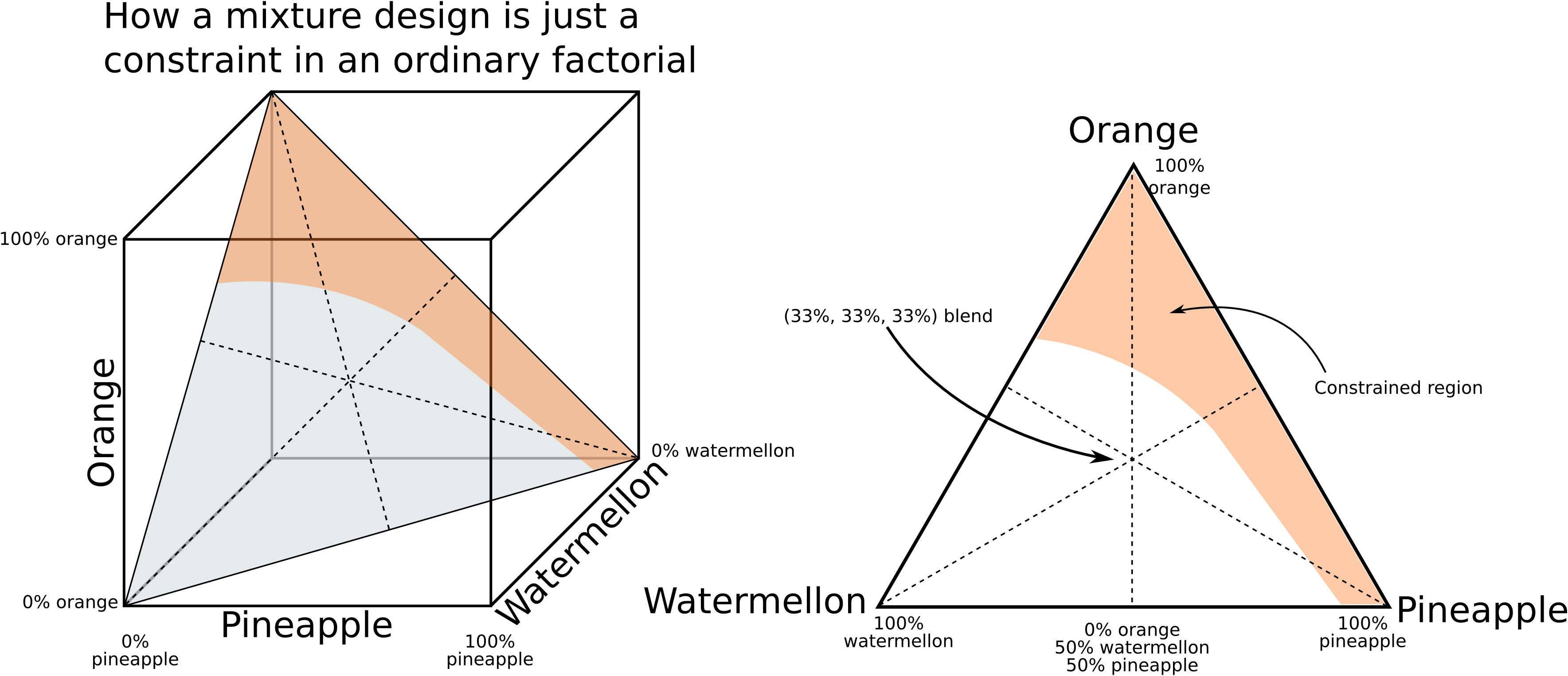
In the above figure on the right, the shaded region represents a constraint that cannot be operated in. A D-optimal algorithm must then be used to select experiments in the remaining region. The example is for finding the lowest cost mixture for a fruit punch, while still meeting certain taste requirements (e.g. watermelon juice is cheap, but has little taste). The constraint represents a region where the acidity is too high.