5.9.7. Saturated designs for screening
A saturated design can be likened to a well trained doctor asking you a few, but very specific, questions to identify a disease or problem. On the other hand, if you sit there just tell the doctor all your symptoms, you may or may not get an accurate diagnosis. Designed experiments, like visiting this doctor, shortens the time required to identify the major effects in a system, and to do so as accurately as possible, within limited budget.
Saturated designs are most suited for screening, and should always be run when you are investigating a new system with many factors. These designs are usually of resolution III and allow you to determine the main effects with a low number of experiments.
For example, a \(2^{7-4}_{\text{III}}\) factorial, introduced in the section on highly fractionated designs, will screen 7 factors in 8 experiments. Once you have run the 8 experiments you can quickly tell which subset of the 7 factors are actually important, and spend the rest of your budget on clearly understanding these effects and their interactions. Bear in mind that there is a risk of confounding, as previously described in that section.
Let’s see how by continuing the previous example, repeated again below with the corresponding values of \(y\). Recall it was a set of eight experiments in seven factors:
Experiment
A
B
C
D=AB
E=AC
F=BC
G=ABC
\(y\)
1
\(-\)
\(-\)
\(-\)
\(+\)
\(+\)
\(+\)
\(-\)
77.1
2
\(+\)
\(-\)
\(-\)
\(-\)
\(-\)
\(+\)
\(+\)
68.9
3
\(-\)
\(+\)
\(-\)
\(-\)
\(+\)
\(-\)
\(+\)
75.5
4
\(+\)
\(+\)
\(-\)
\(+\)
\(-\)
\(-\)
\(-\)
72.5
5
\(-\)
\(-\)
\(+\)
\(+\)
\(-\)
\(-\)
\(+\)
67.9
6
\(+\)
\(-\)
\(+\)
\(-\)
\(+\)
\(-\)
\(-\)
68.5
7
\(-\)
\(+\)
\(+\)
\(-\)
\(-\)
\(+\)
\(-\)
71.5
8
\(+\)
\(+\)
\(+\)
\(+\)
\(+\)
\(+\)
\(+\)
63.7
Use a least squares model to estimate the coefficients in the model:
where \(\mathbf{b} = [b_0, b_A, b_B, b_C, b_D, b_E, b_F, b_G]\). The matrix \(\mathbf{X}\) is essentiall a copy of the above table, but with an added column of 1’s for the intercept term. Notice that the \(\mathbf{X}^T\mathbf{X}\) matrix will be diagonal. Make sure you can calculate \(\mathbf{X}^T\mathbf{X}\) by hand, at least once. It is also straightforward to calculate the solution vector (by hand!), which you can confirm to be \(\mathbf{b} = [70.7, -2.3, 0.1, -2.8, -0.4, 0.5, -0.4, -1.7]\).
How do you assess which main effects are important? There are eight data points and eight parameters, so there are no degrees of freedom and the residuals are all zero. In this case you have to use a Pareto plot, which requires that your variables have been suitably scaled in order to judge importance of the main effects relative to each other. The Pareto plot would be given as shown below, and as usual, it does not show the intercept term.
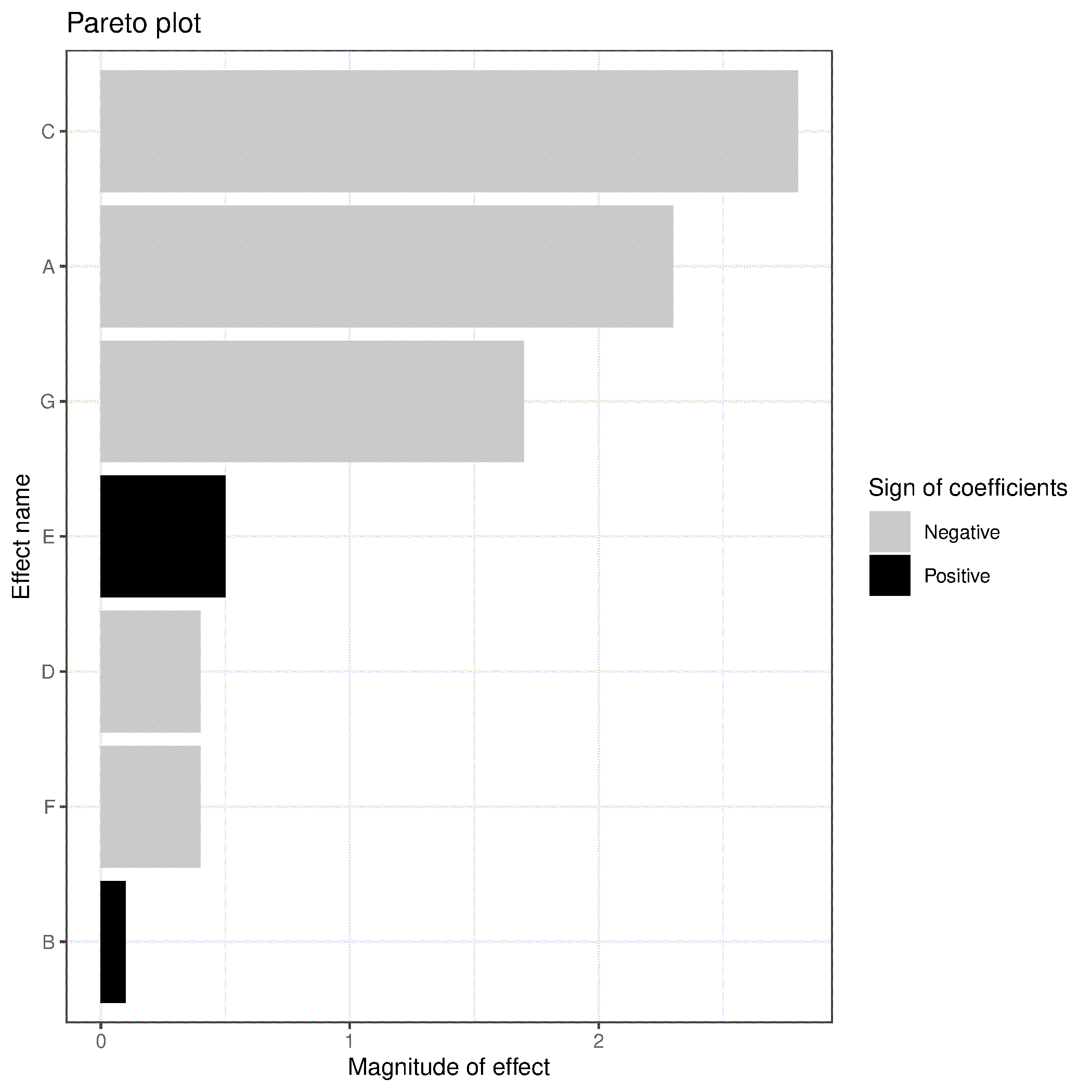
Significant effects would be A, C and G. The next largest effect, E, though fairly small, could be due to the main effect E or due to the AC interaction, because recall the confounding pattern, up to the 2 factor-interactions, for main effect was \(\widehat{\beta}_{\mathbf{E}} \rightarrow\) E + AC + BG + DF.
The factor B is definitely not important to the response variable in this system and can be excluded in future experiments, as could F and D likely. Future experiments should focus on the A, C and G factors and their interactions. We show how to use these existing 8 experiments in the above table, but add a few new ones in the next section on design foldover and by understanding projectivity.
A side note on screening designs is a mention of Plackett and Burman designs. These designs can sometimes be of greater use than a highly fractionated design. A fractional factorial must have \(2^{k-p}\) runs, for integers \(k\) and \(p\): i.e. either \(4, 8, 16, 32, 64, 128, \ldots\) runs. Plackett-Burman designs are screening designs that can be run in any multiple of 4 greater or equal to 12:, i.e. \(12, 16, 20, 24, \ldots\) runs. The Box, Hunter, and Hunter book has more information in Chapter 7, but another interesting paper on these topic is by Box and Bisgaard: “What can you find out from 12 experimental runs?”, which shows how to screen for 11 factors in 12 experiments.
An important mention to readers interested in other, arguable better screening strategies, is to consider definitive screening designs.