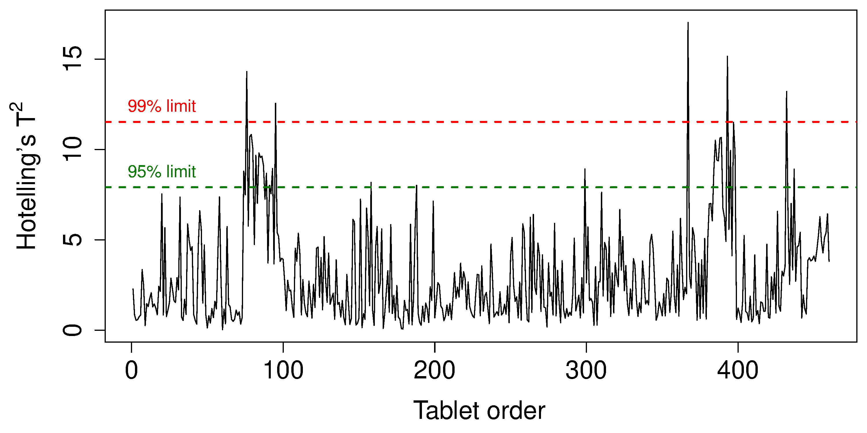
6.5.12. Hotelling’s T²
The final quantity from a PCA model that we need to consider is called Hotelling’s \(T^2\) value. Some PCA models will have many components, \(A\), so an initial screening of these components using score scatterplots will require reviewing \(A(A-1)/2\) scatterplots. The \(T^2\) value for the \(i^\text{th}\) observation is defined as:
where the \(s_a^2\) values are constants, and are the variances of each component. The easiest interpretation is that \(T^2\) is a scalar number that summarizes all the score values. Some other properties regarding \(T^2\):
It is a positive number, greater than or equal to zero.
It is the distance from the center of the (hyper)plane to the projection of the observation onto the (hyper)plane.
An observation that projects onto the model’s center (usually the observation where every value is at the mean), has \(T^2 = 0\).
The \(T^2\) statistic is distributed according to the \(F\)-distribution and is calculated by the multivariate software package being used. For example, we can calculate the 95% confidence limit for \(T^2\), below which we expect, under normal conditions, to locate 95% of the observations.
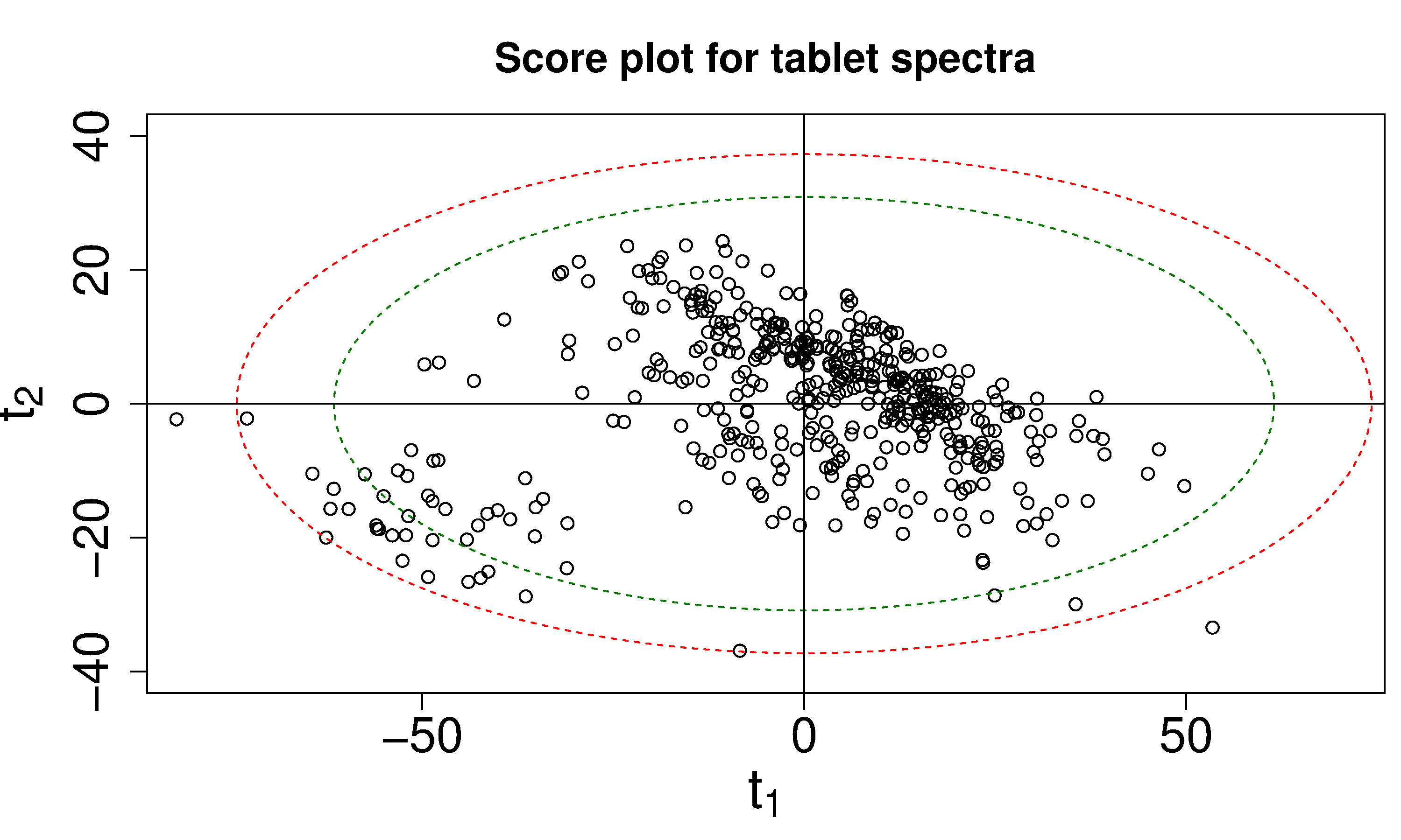
It is useful to consider the case when \(A=2\), and fix the \(T^2\) value at its 95% limit, for example, call that \(T^2_{A=2, \alpha=0.95}\). Using the definition for \(T^2\):
\[T^2_{A=2, \alpha=0.95} = \dfrac{t^2_{1}}{s^2_1} + \dfrac{t^2_{2}}{s^2_2}\]On a scatterplot of \(t_1\) vs \(t_2\) for all observations, this would be the equation of an ellipse, centered at the origin. You will often see this ellipse shown on \(t_i\) vs \(t_j\) scatterplots of the scores. Points inside this elliptical region are within the 95% confidence limit for \(T^2\).
The same principle holds for \(A>2\), except the ellipse is called a hyper-ellipse (think of a rugby-ball shaped object for \(A=3\)). The general interpretation is that if a point is within this ellipse, then it is also below the \(T^2\) limit, if \(T^2\) were to be plotted on a line.