6.7.1. Advantages of the projection to latent structures (PLS) method

So for predictive uses, a PLS model is very similar to principal component regression (PCR) models. And PCR models were a big improvement over using multiple linear regression (MLR). In brief, PCR was shown to have these advantages:

• It handles the correlation among variables in \(\mathbf{X}\) by building a PCA model first, then using those orthogonal scores, \(\mathbf{T}\), instead of \(\mathbf{X}\) in an ordinary multiple linear regression. This prevents us from having to resort to variable selection.

• It extracts these scores \(\mathbf{T}\) even if there are missing values in \(\mathbf{X}\).

• We reduce, but don’t remove, the severity of the assumption in MLR that the predictor’s, \(\mathbf{T}\) in this case, are noise-free. This is because the PCA scores are less noisy than the raw data \(\mathbf{X}\).

• With MLR we require that \(N > K\) (number of observations is greater than the number of variables), but with PCR this is reduced to \(N > A\), and since \(A \ll K\) this requirement is often true, especially for spectral data sets.

• We get the great benefit of a consistency check on the raw data, using SPE and \(T^2\) from PCA, before moving to the second prediction step.

An important point is that PCR is a two-step process:

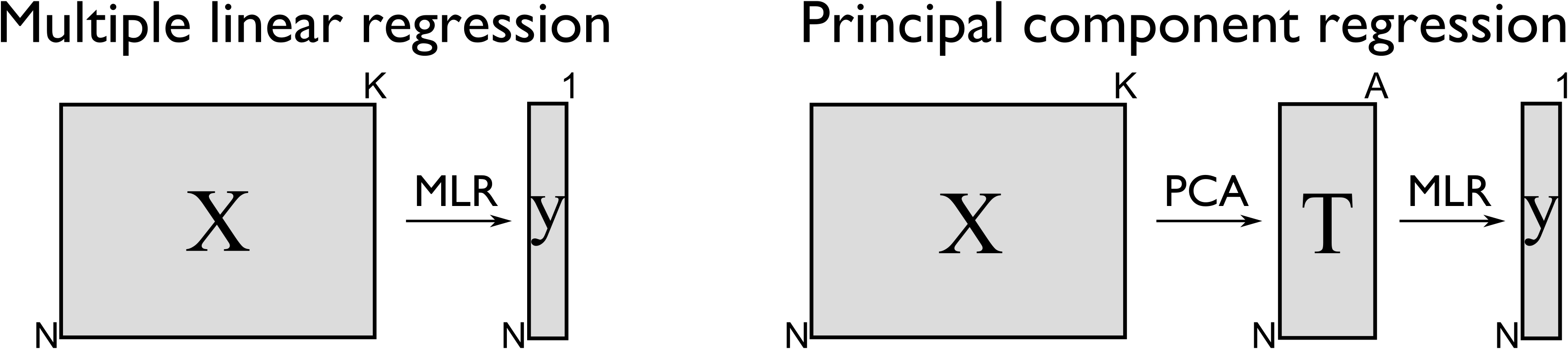
In other words, we replace the \(N \times K\) matrix of raw data with a smaller \(N \times A\) matrix of data that summarizes the original \(\mathbf{X}\) matrix. Then we relate these scores to the \(\mathrm{y}\) variable. Mathematically it is a two-step process:

\[\begin{split}1.&\qquad \mathbf{T} = \mathbf{XP}\\ 2.&\qquad \widehat{\mathbf{y}} = \mathbf{Tb} \qquad \text{and can be solved as}\qquad \mathbf{b} = \left(\mathbf{T'T}\right)^{-1}\mathbf{T'y}\end{split}\]

The PLS model goes a bit further and introduces some additional advantages over PCR:

• A single PLS model can be built for multiple, correlated \(\mathbf{Y}\) variables. This eliminates having to build \(M\) PCR models, one for each column in \(\mathbf{Y}\).

• The PLS model directly assumes that there is error in \(\mathbf{X}\) and \(\mathbf{Y}\). We will return to this important point of an \(\mathbf{X}\)-space model later on.

• PLS is more efficient than PCR in two ways: with PCR, one or more of the score columns in \(\mathbf{T}\) may only have a small correlation with \(\mathbf{Y}\), so these scores are needlessly calculated. Or as is more common, we have to extract many PCA components, going beyond the level of what would normally be calculated (essentially over fitting the PCA model), in order to capture sufficient predictive columns in \(\mathbf{T}\). This augments the size of the PCR model, and makes interpretation harder, which is already strained by the two-step modelling required for PCR.

Similar to PCA, the basis for PCR, we have that PLS also extracts sequential components, but it does so using the data in both \(\mathbf{X}\) and \(\mathbf{Y}\). So it can be seen to be very similar to PCR, but that it calculates the model in one go. From the last point just mentioned, it is not surprising that PLS often requires fewer components than PCR to achieve the same level of prediction. In fact when compared to several regression methods, MLR, ridge regression and PCR, a PLS model is often the most “compact” model.

We will get into the details shortly, but as a starting approximation, you can visualize PLS as a method that extracts a single set of scores, \(\mathbf{T}\), from both \(\mathbf{X}\) and \(\mathbf{Y}\) simultaneously.

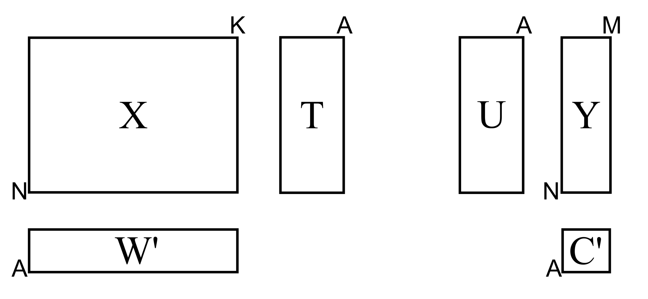
From an engineering point of view this is quite a satisfying interpretation. After all, the variables we chose to be in \(\mathbf{X}\) and in \(\mathbf{Y}\) come from the same system. That system is driven (moved around) by the same underlying latent variables.