6.5.9. Predicted values for each observation

An interesting aspect of a PCA model is that it provides an estimate of each observation in the data set. Recall the latent variable model was oriented to create the best-fit plane to the data. This plane was oriented to minimize the errors, which implies the best estimate of each observation is its perpendicular projection onto the model plane.

Referring to the illustration and assume we have a PCA model with a single component, the best estimate of observation \(\mathbf{x}_i\) is the point along the direction vector, \(\mathbf{p}_1\), where the original observation is projected. Recall that the distance along that direction vector was \(t_{i,1}\), but the actual point along \(\mathbf{p}_1\) is a vector, and it is our best estimate of the original observation. We will call that estimate \(\widehat{\mathbf{x}}_{i,1}\), indicating that it is an estimate of \(\mathbf{x}_i\) along the first component.

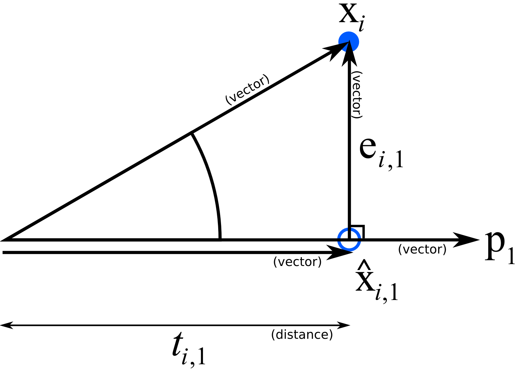
Since \(\widehat{\mathbf{x}}_{i,1}\) is a vector, we can write it as the product of a magnitude value and a direction vector. The magnitude of \(\widehat{\mathbf{x}}_i\) is \(t_i\) in the direction of \(\mathbf{p}_1\), which is a unit vector, then mathematically we can write:

\[\begin{split}\widehat{\mathbf{x}}_{i,1}' &= t_{i,1} \,\,\mathbf{p}'_1 \\ (1 \times K) &= (1 \times 1)(1 \times K)\end{split}\]

This is the best prediction of the original observation using one component. If we added a second component to our model, then our estimate improves:

\[\begin{split}\widehat{\mathbf{x}}_{i,2}' &= t_{i,1}\,\, \mathbf{p}'_1 + t_{i,2}\,\, \mathbf{p}'_2 \\ (1 \times K) &= (1 \times K) + (1 \times K)\end{split}\]

With multiple components, we write:

\[\begin{split}\widehat{\mathbf{x}}_{i,A}' &= \begin{bmatrix}t_{i,1} & t_{i,2}, \,\,\ldots, \,\, t_{i,A} \end{bmatrix} \mathbf{P}'\\ \widehat{\mathbf{x}}_{i,A}' &= \mathbf{t}'_i \, \mathbf{P}'\\ (1 \times K) &= (1 \times A) (A \times K)\end{split}\]

This is interesting: \(\widehat{\mathbf{x}}_{i,A}\) is a prediction of every variable in the \(i^\text{th}\) observation. We only require the score values for that \(i^\text{th}\) observation in order to get this prediction. We multiply the scores \(\mathbf{t}_i\) by the direction vectors in matrix \(\mathbf{P}\) to get the prediction.

The preceding equation can be written in a way that handles the entire matrix \(\mathbf{X}\):

(1)\[\begin{split}\widehat{\mathbf{X}} &= \mathbf{T}\mathbf{P}'\\ (N \times K) &= (N \times A) (A \times K)\end{split}\]

Once we have the predicted value for an observation, we are also interested in the residual vector between the actual and predicted observation:

\[\begin{split}\mathbf{e}'_{i,A} &= \mathbf{x}'_i - \widehat{\mathbf{x}}'_{i,A} \\ (1 \times K) &= (1 \times K) - (1 \times K)\end{split}\]

The residual length or distance is the sum of squares of this residual, then we take the square root to form a distance. Technically the squared prediction error (SPE) is just the sum of squares for each observation, but often we refer to the square root of this quantity as the SPE as well. Some software packages will scale the root of the SPE by some value; you will see this referred to as the DModX, distance to the model plane for \(\mathbf{X}\).

\[\begin{split}\text{SPE}_i &= \sqrt{\mathbf{e}'_{i,A} \mathbf{e}_{i,A}} \\ (1 \times 1) &= (1 \times K)(K \times 1)\end{split}\]

where \(\mathbf{e}_{i,A}\) is the residual vector of the \(i^\text{th}\) observation using \(A\) components.