6.7.7. How the PLS model is calculated
This section assumes that you are comfortable with the NIPALS algorithm for calculating a PCA model from \(\mathbf{X}\). The NIPALS algorithm proceeds in exactly the same way for PLS, except we iterate through both blocks of \(\mathbf{X}\) and \(\mathbf{Y}\).
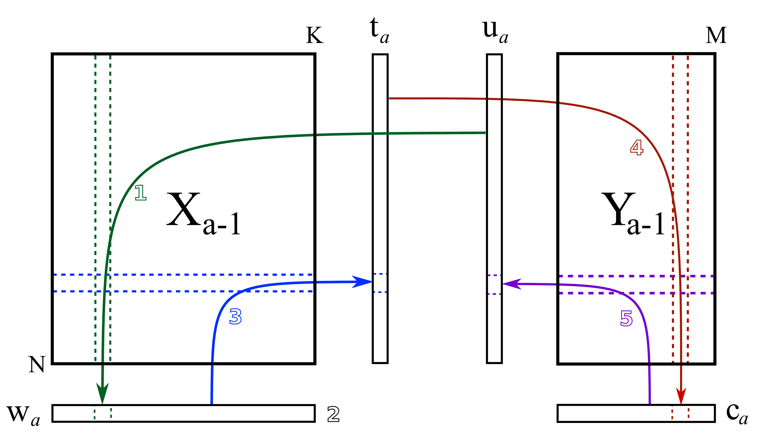
The algorithm starts by selecting a column from \(\mathbf{Y}_a\) as our initial estimate for \(\mathbf{u}_a\). The \(\mathbf{X}_a\) and \(\mathbf{Y}_a\) matrices are just the preprocessed version of the raw data when \(a=1\).
- Arrow 1
Perform \(K\) regressions, regressing each column from \(\mathbf{X}_a\) onto the vector \(\mathbf{u}_a\). The slope coefficients from the regressions are stored as the entries in \(\mathbf{w}_a\). Columns in \(\mathbf{X}_a\) which are strongly correlated with \(\mathbf{u}_a\) will have large weights in \(\mathbf{w}_a\), while unrelated columns will have small, close to zero, weights. We can perform these regression in one go:
\[\mathbf{w}_a = \dfrac{1}{\mathbf{u}'_a\mathbf{u}_a} \cdot \mathbf{X}'_a\mathbf{u}_a\]- Step 2
Normalize the weight vector to unit length: \(\mathbf{w}_a = \dfrac{\mathbf{w}_a}{\sqrt{\mathbf{w}'_a \mathbf{w}_a}}\).
- Arrow 3
Regress every row in \(\mathbf{X}_a\) onto the weight vector. The slope coefficients are stored as entries in \(\mathbf{t}_a\). This means that rows in \(\mathbf{X}_a\) that have a similar pattern to that described by the weight vector will have large values in \(\mathbf{t}_a\). Observations that are totally different to \(\mathbf{w}_a\) will have near-zero score values. These \(N\) regressions can be performed in one go:
\[\mathbf{t}_a = \dfrac{1}{\mathbf{w}'_a\mathbf{w}_a} \cdot \mathbf{X}_a\mathbf{w}_a\]- Arrow 4
Next, regress every column in \(\mathbf{Y}_a\) onto this score vector, \(\mathbf{t}_a\). The slope coefficients are stored in \(\mathbf{c}_a\). We can calculate all \(M\) slope coefficients:
\[\mathbf{c}_a = \dfrac{1}{\mathbf{t}'_a\mathbf{t}_a} \cdot \mathbf{Y}'_a\mathbf{t}_a\]- Arrow 5
Finally, regress each of the \(N\) rows in \(\mathbf{Y}_a\) onto this weight vector, \(\mathbf{c}_a\). Observations in \(\mathbf{Y}_a\) that are strongly related to \(\mathbf{c}_a\) will have large positive or negative slope coefficients in vector \(\mathbf{u}_a\):
\[\mathbf{u}_a = \dfrac{1}{\mathbf{c}'_a\mathbf{c}_a} \cdot \mathbf{Y}_a\mathbf{c}_a\]
This is one round of the NIPALS algorithm. We iterate through these 4 arrow steps until the \(\mathbf{u}_a\) vector does not change much. On convergence, we store these 4 vectors: \(\mathbf{w}_a, \mathbf{t}_a, \mathbf{c}_a\), and \(\mathbf{u}_a\), which jointly define the \(a^{\text{th}}\) component.
Then we deflate. Deflation removes variability already explained from \(\mathbf{X}_a\) and \(\mathbf{Y}_a\). Deflation proceeds as follows:
- Step 1: Calculate a loadings vector for the X space
We calculate the loadings for the \(\mathbf{X}\) space, called \(\mathbf{p}_a\), using the \(\mathbf{X}\)-space scores: \(\mathbf{p}_a = \dfrac{1}{\mathbf{t}'_a\mathbf{t}_a} \cdot \mathbf{X}'_a\mathbf{t}_a\). This loading vector contains the regression slope of every column in \(\mathbf{X}_a\) onto the scores, \(\mathbf{t}_a\). In this regression the \(\mathrm{x}\)-variable is the score vector, and the \(\mathrm{y}\) variable is the column from \(\mathbf{X}_a\). If we want to use this regression model in the usual least squares way, we would need a score vector (our \(\mathrm{x}\)-variable) and predict the column from \(\mathbf{X}_a\) as our \(\mathrm{y}\)-variable.
If this is your first time reading through the notes, you should probably skip ahead to the next step in deflation. Come back to this section after reading about how to use a PLS model on new data, then it will make more sense.
Because it is a regression, it means that if we have a vector of scores, \(\mathbf{t}_a\), in the future, we can predict each column in \(\mathbf{X}_a\) using the corresponding slope coefficient in \(\mathbf{p}_a\). So for the \(k^\text{th}\) column, our prediction of column \(\mathbf{X}_k\) is the product of the slope coefficient, \(p_{k,a}\), and the score vector, \(\mathbf{t}_a\). Or, we can simply predict the entire matrix in one operation: \(\widehat{\mathbf{X}} = \mathbf{t}_a\mathbf{p}'_a\).
Notice that the loading vector \(\mathbf{p}_a\) was calculated after convergence of the 4-arrow steps. In other words, these regression coefficients in \(\mathbf{p}_a\) are not really part of the PLS model, they are merely calculated to later predict the values in the \(\mathbf{X}\)-space. But why can’t we use the \(\mathbf{w}_a\) vectors to predict the \(\mathbf{X}_a\) matrix? Because after all, in arrow step 1 we were regressing columns of \(\mathbf{X}_a\) onto \(\mathbf{u}_a\) in order to calculate regression coefficients \(\mathbf{w}_a\). That would imply that a good prediction of \(\mathbf{X}_a\) would be \(\widehat{\mathbf{X}}_a = \mathbf{u}_a \mathbf{w}'_a\).
That would require us to know the scores \(\mathbf{u}_a\). How can we calculate these? We get them from \(\mathbf{u}_a = \dfrac{1}{\mathbf{c}'_a\mathbf{c}_a} \cdot \mathbf{Y}_a\mathbf{c}_a\). And there’s the problem: the values in \(\mathbf{Y}_a\) are not available when the PLS model is being used in the future, on new data. In the future we will only have the new values of \(\mathbf{X}\). This is why we would rather predict \(\mathbf{X}_a\) using the \(\mathbf{t}_a\) scores, since those \(\mathbf{t}\)-scores are available in the future when we apply the model to new data.
This whole discussion might also leave you asking why we even bother to have predictions of the \(\mathbf{X}\). We do this primarily to ensure orthogonality among the \(\mathbf{t}\)-scores, by removing everything from \(\mathbf{X}_a\) that those scores explain (see the next deflation step).
These predictions of \(\widehat{\mathbf{X}}\) are also used to calculate the squared prediction error, a very important consistency check when using the PLS model on new data.
- Step 2: Remove the predicted variability from X and Y
Using the loadings, \(\mathbf{p}_a\) just calculated above, we remove from \(\mathbf{X}_a\) the best prediction of \(\mathbf{X}_a\), in other words, remove everything we can explain about it.
\[\begin{split}\widehat{\mathbf{X}}_a &= \mathbf{t}_a \mathbf{p}'_a \\ \mathbf{E}_a &= \mathbf{X}_a - \widehat{\mathbf{X}}_a = \mathbf{X}_a - \mathbf{t}_a \mathbf{p}'_a \\ \mathbf{X}_{a+1} &= \mathbf{E}_a\end{split}\]For the first component, the \(\mathbf{X}_{a=1}\) matrix contains the preprocessed raw \(\mathbf{X}\)-data. By convention, \(\mathbf{E}_{a=0}\) is the residual matrix before fitting the first component and is just the same matrix as \(\mathbf{X}_{a=1}\), i.e. the data used to fit the first component.
We also remove any variance explained from \(\mathbf{Y}_a\):
\[\begin{split}\widehat{\mathbf{Y}}_a &= \mathbf{t}_a \mathbf{c}'_a \\ \mathbf{F}_a &= \mathbf{Y}_a - \widehat{\mathbf{Y}}_a = \mathbf{Y}_a - \mathbf{t}_a \mathbf{c}'_a \\ \mathbf{Y}_{a+1} &= \mathbf{F}_a\end{split}\]For the first component, the \(\mathbf{Y}_{a=1}\) matrix contains the preprocessed raw data. By convention, \(\mathbf{F}_{a=0}\) is the residual matrix before fitting the first component and is just the same matrix as \(\mathbf{Y}_{a=1}\).
Notice how in both deflation steps we only use the scores, \(\mathbf{t}_a\), to deflate. The scores, \(\mathbf{u}_a\), are not used for the reason described above: when applying the PLS model to new data in the future, we won’t have the actual \(\mathrm{y}\)-values, which means we also don’t know the \(\mathbf{u}_a\) values.
The algorithm repeats all over again using the deflated matrices for the subsequent iterations.
6.7.7.1. What is the difference between \(\mathbf{W}\) and \(\mathbf{R}\)?
After reading about the NIPALS algorithm for PLS you should be aware that we deflate the \(\mathbf{X}\) matrix after every component is extracted. This means that \(\mathbf{w}_1\) are the weights that best predict the \(\mathbf{t}_1\) score values, our summary of the data in \(\mathbf{X}_{a=1}\) (the preprocessed raw data). Mathematically we can write the following:
The problem comes once we deflate. The \(\mathbf{w}_2\) vector is calculated from the deflated matrix \(\mathbf{X}_{a=2}\), so interpreting these scores is a quite a bit harder.
The \(\mathbf{w}_2\) is not really giving us insight into the relationships between the score, \(\mathbf{t}_2\), and the data, \(\mathbf{X}\), but rather between the score and the deflated data, \(\mathbf{X}_2\).
Ideally we would like a set of vectors we can interpret directly; something like:
One can show, using repeated substitution, that a matrix \(\mathbf{R}\), whose columns contain \(\mathbf{r}_a\), can be found from: \(\mathbf{R} = \mathbf{W}\left(\mathbf{P}'\mathbf{W}\right)^{-1}\). The first column, \(\mathbf{r}_1 = \mathbf{w}_1\).
So our preference is to interpret the \(\mathbf{R}\) weights (often called \(\mathbf{W}^*\) in some literature), rather than the \(\mathbf{W}\) weights when investigating the relationships in a PLS model.