4.13. Exercises

Show all answers

Question 1

Use the distillation column data set and choose any two variables, one for \(\mathrm{x}\) and one as \(\mathrm{y}\). Then fit the following models by least squares in any software package you prefer:

• \(y_i = b_0 + b_1 x_i\)

• \(y_i = b_0 + b_1 (x_i - \overline{x})\) (what does the \(b_0\) coefficient represent in this case?)

• \((y_i - \overline{y}) = b_0 + b_1 (x_i - \overline{x})\)

Prove to yourself that centering the \(\mathrm{x}\) and \(\mathrm{y}\) variables gives the same model for the 3 cases in terms of the \(b_1\) slope coefficient, standard errors and other model outputs.

Solution Click to show answer

Once you have created an x and y variable in R, compare the output from these 3 models:

# Model 1
summary(lm(y ~ x))

# Model 2
x.mc <- x - mean(x)
summary(lm(y ~ x.mc))

# Model 3
y.mc <- y - mean(y)
summary(lm(y.mc ~ x.mc))

Question 2

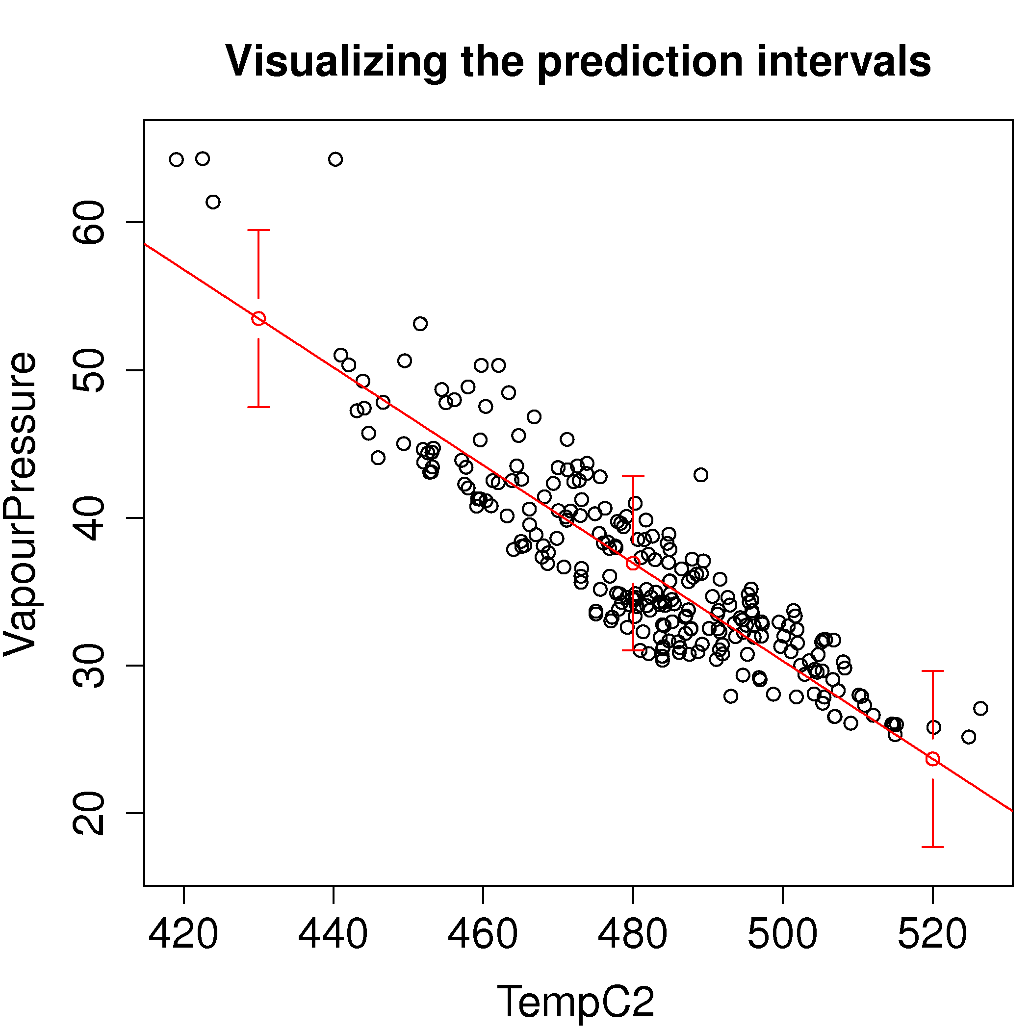
For a \(x_{\text{new}}\) value and the linear model \(y = b_0 + b_1 x\) the prediction interval for \(\hat{y}_\text{new}\) is:

\[\hat{y}_i \pm c_t \sqrt{V\{\hat{y}_i\}}\]

where \(c_t\) is the critical t-value, for example at the 95% confidence level.

Use the distillation column data set and with \(\mathrm{y}\) as VapourPressure (units are kPa) and \(\mathrm{x}\) as TempC2 (units of degrees Farenheit) fit a linear model. Calculate the prediction interval for vapour pressure at these 3 temperatures: 430, 480, 520 °F.

Solution Click to show answer

The prediction interval is dependent on the value of \(x_\text{new, i}\) used to make the prediction. For this model, \(S_E = 2.989\) kPa, \(n=253\), \(\sum_j{(x_j - \overline{x})^2} = 86999.6\), and \(\overline{x} = 480.82\).

\[\mathcal{V}\left(\hat{y}_\text{new,i}\right) = S_E^2 \left(1 + \dfrac{1}{n} + \dfrac{\left(x_\text{new}-\overline{x}\right)^2}{ \sum_j{(x_j - \overline{x})^2}} \right)\]

Calculating this term manually, or using the predict(model, newdata=..., int="p") function in R gives the 95% prediction interval:

• \(x_\text{new} = 430\) °F: \(\hat{y}_\text{new} = 53.49 \pm 11.97\), or [47.50, 59.47]

• \(x_\text{new} = 480\) °F: \(\hat{y}_\text{new} = 36.92 \pm 11.80\), or [31.02, 42.82]

• \(x_\text{new} = 520\) °F: \(\hat{y}_\text{new} = 23.67 \pm 11.90\), or [17.72, 29.62]

dist <- read.csv('http://openmv.net/file/distillation-tower.csv')
attach(dist)
model <- lm(VapourPressure ~ TempC2)
summary(model)

# From the above output
SE = sqrt(sum(resid(model)^2)/model$df.residual)
n = length(TempC2)
k = model$rank
x.new = data.frame(TempC2 = c(430, 480, 520))
x.bar = mean(TempC2)
x.variance = sum((TempC2-x.bar)^2)
var.y.hat = SE^2 * (1 + 1/n + (x.new-x.bar)^2/x.variance)
c.t = -qt(0.025, df=n-k)
y.hat = predict(model, newdata=x.new, int="p")
PI.LB = y.hat[,1] - c.t*sqrt(var.y.hat)
PI.UB = y.hat[,1] + c.t*sqrt(var.y.hat)

# Results from y.hat agree with PI.LB and PI.UB
y.hat
#        fit      lwr      upr
# 1 53.48817 47.50256 59.47379
# 2 36.92152 31.02247 42.82057
# 3 23.66819 17.71756 29.61883
y.hat[,3] - y.hat[,2]
plot(TempC2, VapourPressure, ylim = c(17, 65), main="Visualizing the prediction intervals")
abline(model, col="red")
library(gplots)
plotCI(x=c(430, 480, 520), y=y.hat[,1], li=y.hat[,2], ui=y.hat[,3], add=TRUE, col="red")

Question 3

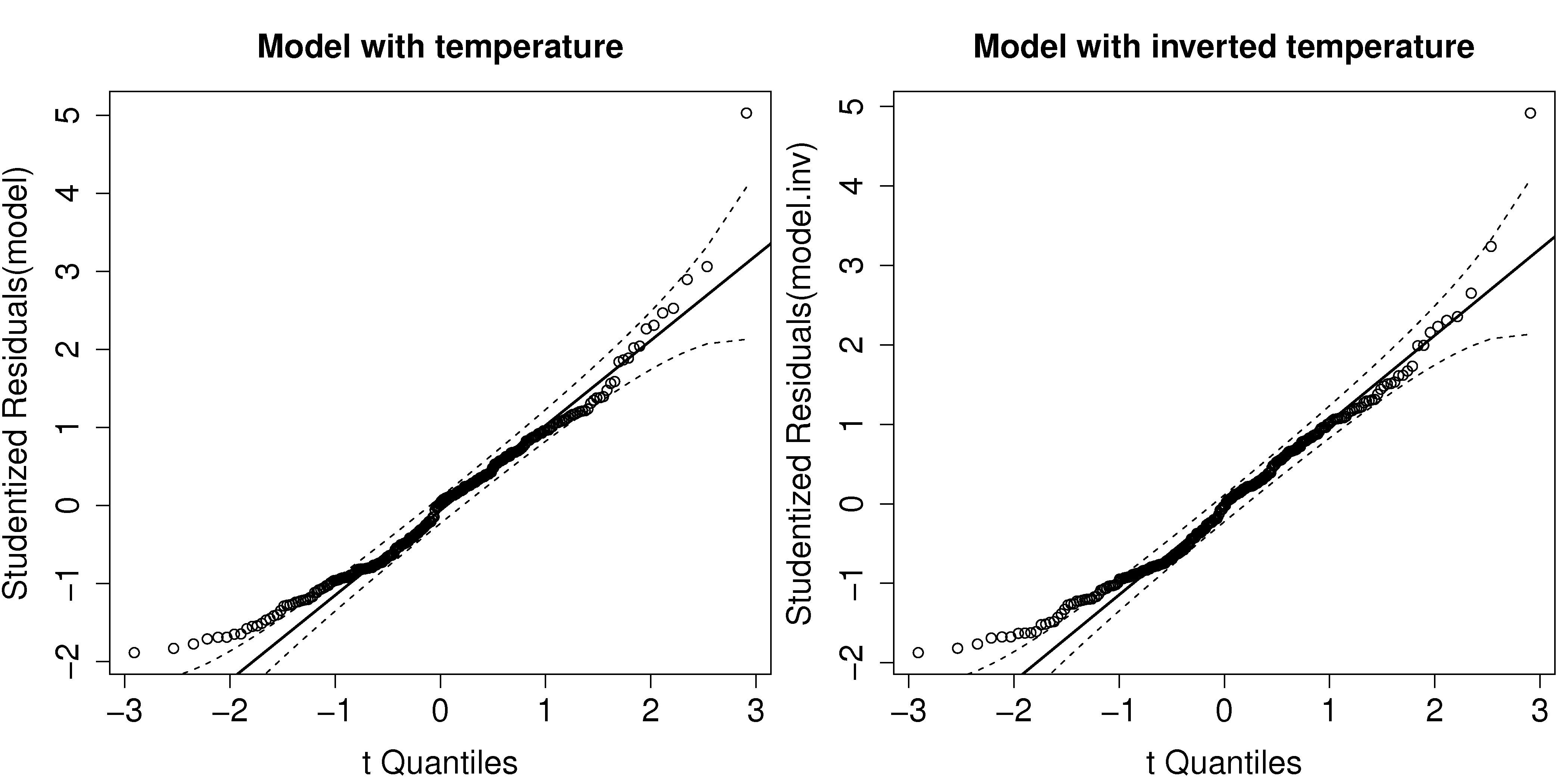
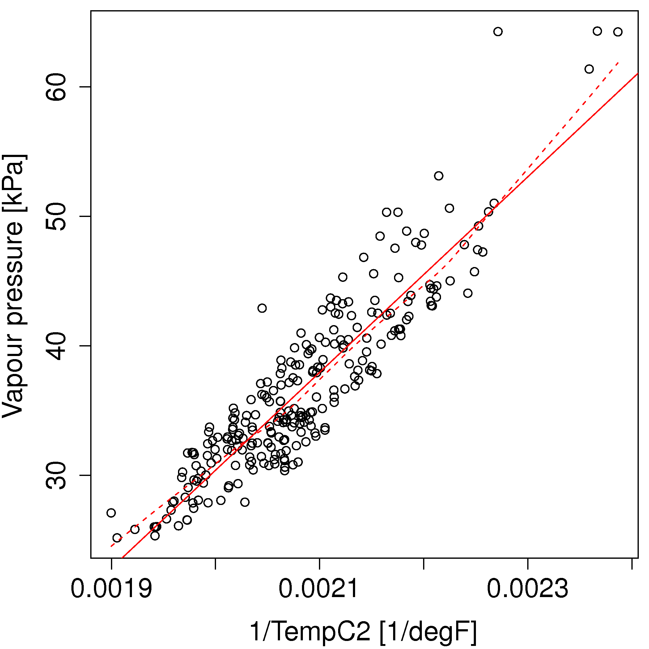
Refit the distillation model from the previous question with a transformed temperature variable. Use \(1/T\) instead of the actual temperature.

• Does the model fit improve?

• Are the residuals more normally distributed with the untransformed or transformed temperature variable?

• How do you interpret the slope coefficient for the transformed temperature variable?

• Use the model to compute the predicted vapour pressure at a temperature of 480 °F, and also calculate the corresponding prediction interval at that new temperature.

Solution Click to show answer

• Using the model.inv <- lm(VapourPressure ~ I(1/TempC2)) instruction, one obtains the model summary below. The model fit has improved slightly: the standard error is 2.88 kPa, reduced from 2.99 kPa.

  Call:
  lm(formula = VapourPressure ~ I(1/TempC2))
  
  Residuals:
       Min       1Q   Median       3Q      Max
  -5.35815 -2.27855 -0.08518  1.95057 13.38436
  
  Coefficients:
               Estimate Std. Error t value Pr(>|t|)
  (Intercept)  -120.760      4.604  -26.23   <2e-16 ***
  I(1/TempC2) 75571.306   2208.631   34.22   <2e-16 ***
  ---
  Signif. codes:  0 ‘***’ 0.001 ‘**’ 0.01 ‘*’ 0.05 ‘.’ 0.1 ‘ ’ 1
  
  Residual standard error: 2.88 on 251 degrees of freedom
  Multiple R-squared: 0.8235,     Adjusted R-squared: 0.8228
  F-statistic:  1171 on 1 and 251 DF,  p-value: < 2.2e-16
  

• The residuals have roughly the same distribution as before, maybe a little more normal on the left tail, but hardly noticeable.

  

• The slope coefficient of 75571 has units of kPa.°F, indicating that each one unit decrease in temperature results in an increase in vapour pressure. Since division is not additive, the change in vapour pressure when decreasing 10 degrees from 430 °F is a different decrease to that when temperature is 530 °F. The interpretation of transformed variables in linear models is often a lot harder. The easiest interpretation is to show a plot of 1/T against vapour pressure.

  

• The predicted vapour pressure at 480 °F is 36.68 kPa \(\pm 11.37\), or within the range [31.0 to 42.4] with 95% confidence, very similar to the prediction interval from question 2.

# Model with inverted temperature
model.inv <- lm(VapourPressure ~ I(1/TempC2))
summary(model.inv)

plot(1/TempC2, VapourPressure, xlab="1/TempC2 [1/degF]", ylab="Vapour pressure [kPa]")
abline(model.inv, col="red")
lines(lowess(1/TempC2, VapourPressure), lty=2, col="red")

x.new = data.frame(TempC2 = c(430, 480, 520))
y.hat = predict(model.inv, newdata=x.new, int="p")
y.hat
#        fit      lwr      upr
# 1 54.98678 49.20604 60.76751
# 2 36.67978 30.99621 42.36334
# 3 24.56899 18.84305 30.29493

layout(matrix(c(1,2), 1, 2))
library(car)
qqPlot(model, main="Model with temperature", col=c(1, 1))
qqPlot(model.inv, main="Model with inverted temperature",col=c(1, 1))

Question 4

Again, for the distillation model, use the data from 2000 and 2001 to build the model (the first column in the data set contains the dates). Then use the remaining data to test the model. Use \(\mathrm{x}\) = TempC2 and \(\mathrm{y}\) = VapourPressure in your model.

• Calculate the RMSEP for the testing data. How does it compare to the standard error from the model?

• Now use the influencePlot(...) function from the car library, to highlight the influential observations in the model building data (2000 and 2001). Show your plot with observation labels (observation numbers are OK). See part 5 of the R tutorial for some help.

• Explain how the points you selected are influential on the model?

• Remove these influential points, and refit the model on the training data. How has the model’s slope and standard error changed?

• Recalculate the RMSEP for the testing data; how has it changed?

Short answer: Click to show answerRMSEP = 4.18 kPa; standard error = 2.68 kPa.

Question 5

The Kappa number data set was used in an earlier question to construct a Shewhart chart. The “Mistakes to avoid” section (Process Monitoring), warns that the subgroups for a Shewhart chart must be independent to satisfy the assumptions used to derived the Shewhart limits. If the subgroups are not independent, then it will increase the type I (false alarm) rate.

This is no different to the independence required for least squares models. Use the autocorrelation tool to determine a subgroup size for the Kappa variable that will satisfy the Shewhart chart assumptions. Show your autocorrelation plot and interpret it as well.

Question 6

You presume the yield from your lab-scale bioreactor, \(y\), is a function of reactor temperature, batch duration, impeller speed and reactor type (one with with baffles and one without). You have collected these data from various experiments.

Temp = \(T\) [°C]	Duration = \(d\) [minutes]	Speed = \(s\) [RPM]	Baffles = \(b\) [Yes/No]	Yield = \(y\) [g]
82	260	4300	No	51
90	260	3700	Yes	30
88	260	4200	Yes	40
86	260	3300	Yes	28
80	260	4300	No	49
78	260	4300	Yes	49
82	260	3900	Yes	44
83	260	4300	No	59
64	260	4300	No	60
73	260	4400	No	59
60	260	4400	No	57
60	260	4400	No	62
101	260	4400	No	42
92	260	4900	Yes	38

• Use software to fit a linear model that predicts the yield from these variables (the data set is available from the website). See the R tutorial for building linear models with integer variables in R.

• Interpret the meaning of each effect in the model. If you are using R, then the confint(...) function will be helpful as well. Show plots of each \(\mathrm{x}\) variable in the model against yield. Use a box plot for the baffles indicator variable.

• Now calculate the \(\mathbf{X}^T\mathbf{X}\) and \(\mathbf{X}^T\mathbf{y}\) matrices; include a column in the \(\mathbf{X}\) matrix for the intercept. Since you haven’t mean centered the data to create these matrices, it would be misleading to try interpret them.

• Calculate the least squares model estimates from these two matrices. See the R tutorial for doing matrix operations in R, but you might prefer to use MATLAB for this step. Either way, you should get the same answer here as in the first part of this question.

Question 7

In the section on comparing differences between two groups we used, without proof, the fact that:

\[\mathcal{V}\left\{\overline{x}_B - \overline{x}_A\right\} = \mathcal{V}\left\{\overline{x}_B\right\} + \mathcal{V}\left\{\overline{x}_A\right\}\]

Prove this statement, and clearly explain all steps in your proof.

Question 8

The production of low density polyethylene is carried out in long, thin pipes at high temperature and pressure (1.5 kilometres long, 50mm in diameter, 500 K, 2500 atmospheres). One quality measurement of the LDPE is its melt index. Laboratory measurements of the melt index can take between 2 to 4 hours. Being able to predict this melt index, in real time, allows for faster adjustment to process upsets, reducing the product’s variability. There are many variables that are predictive of the melt index, but in this example we only use a temperature measurement that is measured along the reactor’s length.

These are the data of temperature (K) and melt index (units of melt index are “grams per 10 minutes”).

Temperature = \(T\) [Kelvin]	441	453	461	470	478	481	483	485	499	500	506	516
Melt index = \(m\) [g per 10 mins]	9.3	6.6	6.6	7.0	6.1	3.5	2.2	3.6	2.9	3.6	4.2	3.5

The following calculations have already been performed:

• Number of samples, \(n = 12\)

• Average temperature = \(\overline{T} = 481\) K

• Average melt index, \(\overline{m} = 4.925\) g per 10 minutes.

• The summed product, \(\sum_i{\left(T_i-\overline{T}\right)\left(m_i - \overline{m}\right)} = -422.1\)

• The sum of squares, \(\sum_i{\left(T_i-\overline{T}\right)^2} = 5469.0\)

1. Use this information to build a predictive linear model for melt index from the reactor temperature.

2. What is the model’s standard error and how do you interpret it in the context of this model? You might find the following software software output helpful, but it is not required to answer the question.

   Call:
   lm(formula = Melt.Index ~ Temperature)
   
   Residuals:
       Min      1Q  Median      3Q     Max
   -2.5771 -0.7372  0.1300  1.2035  1.2811
   
   Coefficients:
               Estimate Std. Error t value Pr(>|t|)
   (Intercept) --------    8.60936   4.885 0.000637
   Temperature --------    0.01788  -4.317 0.001519
   
   Residual standard error: 1.322 on 10 degrees of freedom
   Multiple R-squared: 0.6508,     Adjusted R-squared: 0.6159
   F-statistic: 18.64 on 1 and 10 DF,  p-value: 0.001519
   

3. Quote a confidence interval for the slope coefficient in the model and describe what it means. Again, you may use the above software output to help answer your question.

Short answer: Click to show answerm = 42.0 - 0.0772 T

Question 9

For a distillation column, it is well known that the column temperature directly influences the purity of the product, and this is used in fact for feedback control, to achieve the desired product purity. Use the distillation data set , and build a least squares model that predicts VapourPressure from the temperature measurement, TempC2. Report the following values:

1. the slope coefficient, and describe what it means in terms of your objective to control the process with a feedback loop

2. the interquartile range and median of the model’s residuals

3. the model’s standard error

4. a confidence interval for the slope coefficient, and its interpretation.

You may use any computer package to build the model and read these values off the computer output.

Question 10

Use the bioreactor data, which shows the percentage yield from the reactor when running various experiments where temperature was varied, impeller speed and the presence/absence of baffles were adjusted.

1. Build a linear model that uses the reactor temperature to predict the yield. Interpret the slope and intercept term.

2. Build a linear model that uses the impeller speed to predict yield. Interpret the slope and intercept term.

3. Build a linear model that uses the presence (represent it as 1) or absence (represent it as 0) of baffles to predict yield. Interpret the slope and intercept term.

   Note: if you use R it will automatically convert the baffles variable to 1’s and 0’s for you. If you wanted to make the conversion yourself, to verify what R does behind the scenes, try this:

   # Read in the data frame
   bio <- read.csv('http://openmv.net/file/bioreactor-yields.csv')
   
   # Force the baffles variables to 0's and 1's
   bio$baffles <- as.numeric(bio$baffles) - 1
   

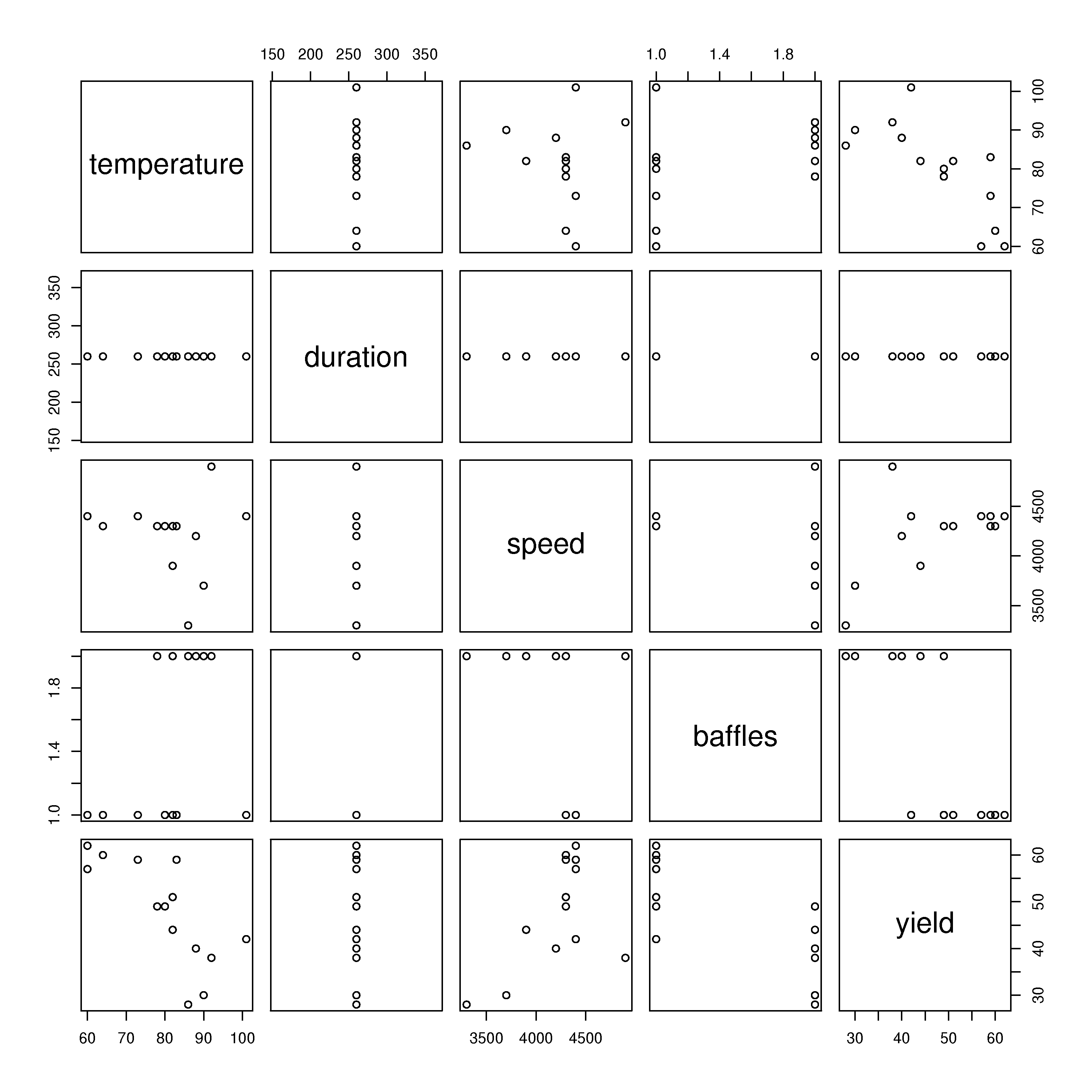
4. Which variable(s) would you change to boost the batch yield, at the lowest cost of implementation?

5. Use the plot(bio) function in R, where bio is the data frame you loaded using the read.csv(...) function. R notices that bio is not a single variable, but a group of variables, i.e. a data frame, so it plots what is called a scatterplot matrix instead. Describe how the scatterplot matrix agrees with your interpretation of the slopes in parts 1, 2 and 3 of this question.

Solution Click to show answer

The R code (below) was used to answer all questions.

1. • The model is: \(\hat{y} = 102.5 - 0.69T\), where \(T\) is tank temperature.

   • Intercept = \(102.5\) % points is the yield when operating at 0 \(^\circ \text{C}\). Obviously not a useful interpretation, because data have not been collected in a range that spans, or is even close to 0 \(^\circ \text{C}\). It is likely that this bioreactor system won’t yield any product under such cold conditions. Further, a yield greater than 100% is not realizable.

   • Slope = -0.69 \(\frac{[\%]}{[^\circ \text{C}]}\), indicating the yield decreases, on average, by about 0.7 units for every degree increase in tank temperature.

2. • The model is: \(\hat{y} = -20.3 + 0.016S\), where \(S\) is impeller speed.

   • Intercept = \(-20.3\) % points is the yield when operating no agitation. Again, obviously not a useful interpretation, because the data have not been collected under these conditions, and yield can’t be a negative quantity.

   • Slope = 0.016 \(\frac{[\%]}{[\text{RPM}]}\), indicating the yield increases, on average, by about 1.6 percentage points per 100 RPM increase.

3. • The model is: \(\hat{y} = 54.9 - 16.7B\), where \(B\) is 1 if baffles are present and \(B=0\) with no baffles.

   • Intercept = \(54.9\) % points yield is the yield when operating with no baffles (it is in fact the average yield of all the rows that have “No” as their baffle value).

   • Slope = -16.7 %, indicating the presence of baffles decreases the yield, on average, by about 16.7 percentage points.

4. This is an open-ended, and case specific. Some factors you would include are:

   • Remove the baffles, but take into account the cost of doing so. Perhaps it takes a long time (expense) to remove them, especially if the reactor is used to produce other products that do require the baffles.

   • Operate at lower temperatures. The energy costs of cooling the reactor would factor into this.

   • Operate at higher speeds and take that cost into account. Notice however there is one observation at 4900 RPM that seems unusual: was that due to the presence of baffles, or due to temperature in that run? We’ll look into this issue with multiple linear regression later on.

   Note

   Please note that our calculations above are not the true effect of each of the variables (temperature, speed and baffles) on yield. Our calculations assume that there is no interaction between temperature, speed and baffles, and that each effect operates independent of the others. That’s not necessarily true. See the section on interpreting MLR coefficients to learn how to “control for the effects” of other variables.

5. The scatterplot matrix, shown below, agrees with our interpretation. This is an information rich visualization that gives us a feel for the multivariate relationships and really summarizes all the variables well (especially the last row of plots).

   • The yield-temperature relationship is negative, as expected.

   • The yield-speed relationship is positive, as expected.

   • The yield-baffles relationship is negative, as expected.

   • We can’t tell anything about the yield-duration relationship, as it doesn’t vary in the data we have (there could/should be a relationship, but we can’t tell).

   

bio <- read.csv('http://openmv.net/file/bioreactor-yields.csv')
summary(bio)

# Temperature-Yield model
model.temp <- lm(bio$yield ~ bio$temperature)
summary(model.temp)

# Impeller speed-Yield model
model.speed <- lm(bio$yield ~ bio$speed)
summary(model.speed)

# Baffles-Yield model
model.baffles <- lm(bio$yield ~ bio$baffles)
summary(model.baffles)

# Scatterplot matrix
bitmap('bioreactor-scatterplot-matrix.png', type="png256", 
        width=10, height=10, res=300)
plot(bio)
dev.off()

Question 11

Use the gas furnace data from the website to answer these questions. The data represent the gas flow rate (centered) from a process and the corresponding CO₂ measurement.

1. Make a scatter plot of the data to visualize the relationship between the variables. How would you characterize the relationship?

2. Calculate the variance for both variables, the covariance between the two variables, and the correlation between them, \(r(x,y)\). Interpret the correlation value; i.e. do you consider this a strong correlation?

3. Now calculate a least squares model relating the gas flow rate as the \(x\) variable to the CO₂ measurement as the \(y\)-variable. Report the intercept and slope from this model.

4. Report the \(R^2\) from the regression model. Compare the squared value of \(r(x,y)\) to \(R^2\). What do you notice? Now reinterpret what the correlation value means (i.e. compare this interpretation to your answer in part 2).

5. Advanced: Switch \(x\) and \(y\) around and rebuild your least squares model. Compare the new \(R^2\) to the previous model’s \(R^2\). Is this result surprising? How do interpret this?

Question 12

A new type of thermocouple is being investigated by your company’s process control group. These devices produce an almost linear voltage (millivolt) response at different temperatures. In practice though it is used the other way around: use the millivolt reading to predict the temperature. The process of fitting this linear model is called calibration.

1. Use the following data to calibrate a linear model:

   Temperature [K]	273	293	313	333	353	373	393	413	433	453
   Reading [mV]	0.01	0.12	0.24	0.38	0.51	0.67	0.84	1.01	1.15	1.31

   Show the linear model and provide the predicted temperature when reading 1.00 mV.

2. Are you satisfied with this model, based on the coefficient of determination (\(R^2\)) value?

3. What is the model’s standard error? Now, are you satisfied with the model’s prediction ability, given that temperatures can usually be recorded to an accuracy of \(\pm 0.5\) K with most inexpensive thermocouples.

4. What is your (revised) conclusion now about the usefulness of the \(R^2\) value?

Note: This example explains why we don’t use the terminology of independent and dependent variables in this book. Here the temperature truly is the independent variable, because it causes the voltage difference that we measure. But the voltage reading is the independent variable in the least squares model. The word independent is being used in two different senses (its English meaning vs its mathematical meaning), and this can be misleading.

Question 13

1. Use the linear model you derived in the gas furnace question, where you used the gas flow rate to predict the CO₂ measurement, and construct the analysis of variance table (ANOVA) for the dataset. Use your ANOVA table to reproduce the residual standard error, \(S_E\) value, that you get from the R software output.

   Go through the R tutorial to learn how to efficiently obtain the residuals and predicted values from a linear model object.

2. Also for the above linear model, verify whether the residuals are normally distributed.

3. Use the linear model you derived in the thermocouple question, where you used the voltage measurement to predict the temperature, and construct the analysis of variance table (ANOVA) for that dataset. Use your ANOVA table to reproduce the residual standard error, \(S_E\) value, that you get from the R software output.

Solution Click to show answer

1. The ANOVA table values were calculated in the code solutions for question 2:

   Type of variance	Distance	Degrees of freedom	SSQ	Mean square
   Regression	\(\hat{y}_i - \overline{\mathrm{y}}\)	\(k-2\)	709.9	354.9
   Error	\(y_i - \hat{y}_i\)	\(n-k\)	2314.9	7.87
   Total	\(y_i - \overline{\mathrm{y}}\)	\(n\)	3024.8	10.2

   The residual standard error, or just standard error, \(S_E = \sqrt{\frac{2314.9}{296-2}} = 2.8\) %CO₂, which agrees with the value from R.

2. These residuals were normally distributed, as verified in the q-q plot:

   

   As mentioned in the help(qqPlot) output, the dashed red line is the confidence envelope at the 95% level. The single point just outside the confidence envelope is not going to have any practical effect on our assumption of normality. We expect 1 point in 20 to lie outside the limits.

   Read ahead, if required, on the meaning of studentized residuals, which are used on the \(y\)-axis.

3. For the thermocouple data set:

   Type of variance	Distance	Degrees of freedom	SSQ	Mean square
   Regression	\(\hat{y}_i - \overline{\mathrm{y}}\)	\(k-2\)	32877	16438
   Error	\(y_i - \hat{y}_i\)	\(n-k\)	122.7	15.3
   Total	\(y_i - \overline{\mathrm{y}}\)	\(n\)	33000	3300

   The residual standard error, or just standard error, \(S_E = \sqrt{\frac{122.7}{10-2}} = 3.9\) K, which agrees with the value from R.

Question 14

Use the mature cheddar cheese data set for this question.

1. Choose any \(x\)-variable, either Acetic acid concentration (already log-transformed), H2S concentration (already log-transformed), or Lactic acid concentration (in original units) and use this to predict the Taste variable in the data set. The Taste is a subjective measurement, presumably measured by a panel of tasters.

   Prove that you get the same linear model coefficients, \(R^2\), \(S_E\) and confidence intervals whether or not you first mean center the \(x\) and \(y\) variables.

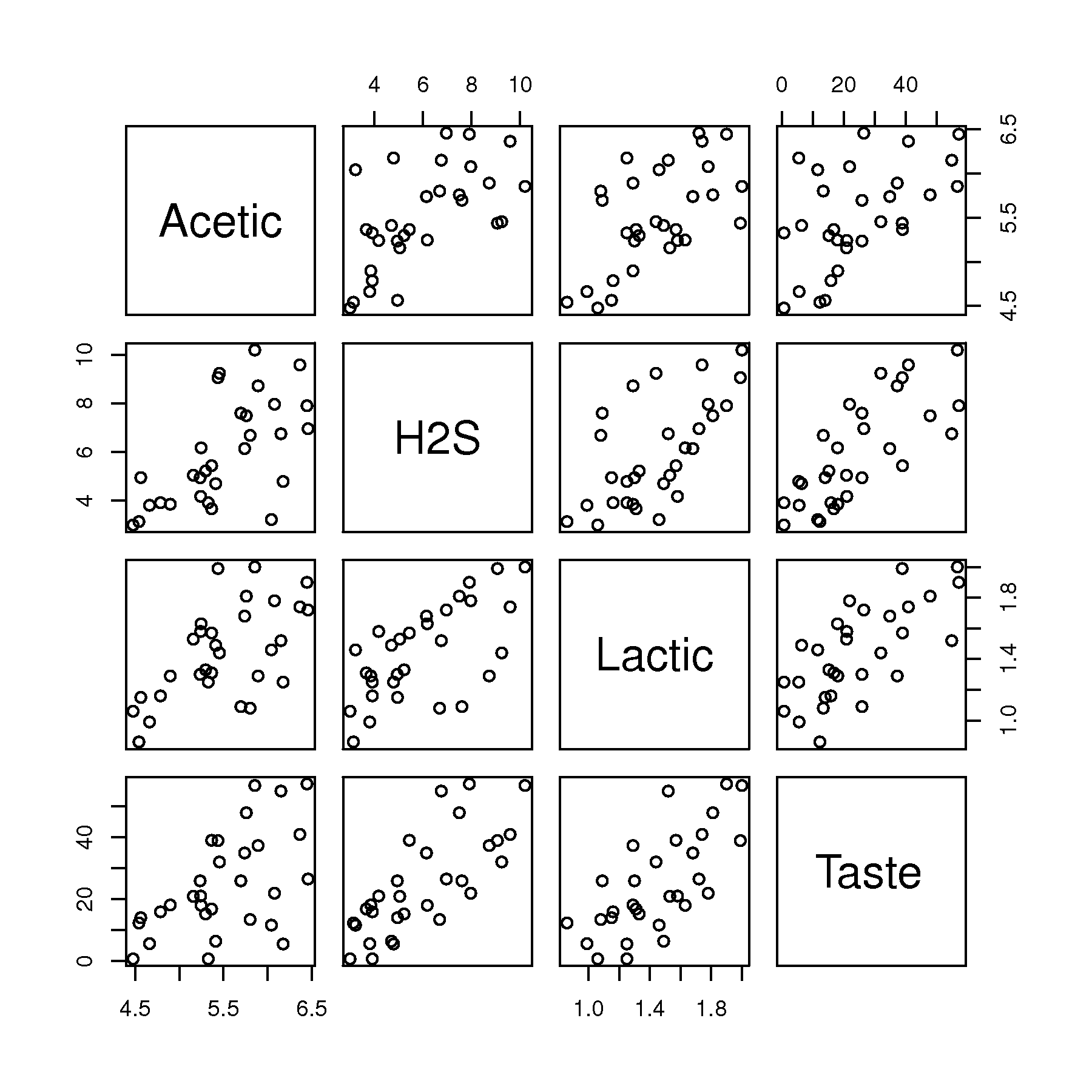
2. What is the level of correlation between each of the \(x\)-variables. Also show a scatterplot matrix to learn what this level of correlation looks like visually.

   • Report your correlations as a \(3 \times 3\) matrix, where there should be 1.0’s on the diagonal, and values between \(-1\) and \(+1\) on the off-diagonals.

3. Build a linear regression that uses all three \(x\)-variables to predict \(y\).

   • Report the slope coefficient and confidence interval for each \(x\)-variable

   • Report the model’s standard error. Has it decreased from the model in part 1?

   • Report the model’s \(R^2\) value. Has it decreased?

Solution Click to show answer

1. We used the acetic acid variable as \(x\) and derived the following two models to predict taste, \(y\):

   • No mean centering of \(x\) and \(y\): \(y = -61.5 + 15.65x\)

   • With mean centering of \(x\) and \(y\): \(y = 0 + 15.65x\)

   These results were found from both models:

   • Residual standard error, \(S_E\) = 13.8 on 28 degrees of freedom

   • Multiple R-squared, \(R^2\) = 0.30

   • Confidence interval for the slope, \(b_a\) was: \(6.4 \leq b_A \leq 24.9\).

   Please see the R code at the end of this question.

   If you had used \(x\) = H2S, then \(S_E = 10.8\) and if used \(x\) = Lactic, then \(S_E = 11.8\).

2. The visual level of correlation is shown in the first \(3 \times 3\) plots below, while the relationship of each \(x\) to \(y\) is shown in the last row and column:

   

   The numeric values for the correlation between the \(x\)-variables are:

   \[\begin{split}\begin{bmatrix} 1.0 & 0.618 & 0.604\\ 0.618 & 1.0 & 0.644\\ 0.604 & 0.644 & 1.0 \end{bmatrix}\end{split}\]

   There is about a 60% correlation between each of the \(x\)-variables in this model, and in each case the correlation is positive.

3. A combined linear regression model is \(y = -28.9 + 0.31 x_A + 3.92 x_S + 19.7 x_L\) where \(x_A\) is the log of the acetic acid concentration, \(x_S\) is the log of the hydrogen sulphide concentration and \(x_L\) is the lactic acid concentration in the cheese. The confidence intervals for each coefficient are:

   • \(-8.9 \leq b_A \leq 9.4\)

   • \(1.4 \leq b_S \leq 6.5\)

   • \(1.9 \leq b_A \leq 37\)

   The \(R^2\) value is 0.65 in the MLR, compared to the value of 0.30 in the single variable regression. The \(R^2\) value will always decrease when adding a new variable to the model, even if that variable has little value to the regression model (yet another caution related to \(R^2\)).

   The MLR standard error is 10.13 on 26 degrees of freedom, a decrease of about 3 units from the individual regression in part 1; a small decrease given the \(y\)-variable’s range of about 50 units.

   Since each \(x\)-variable is about 60% correlated with the others, we can loosely interpret this by inferring that either lactic, or acetic or H2S could have been used in a single-variable regression. In fact, if you compare \(S_E\) values for the single-variable regressions, (13.8, 10.8 and 11.8), to the combined regression \(S_E\) of 10.13, there isn’t much of a reduction in the MLR’s standard error.

   This interpretation can be quite profitable: it means that we get by with one only one \(x\)-variable to make a reasonable prediction of taste in the future, however, the other two measurements must be consistent. In other words we can pick lactic acid as our predictor of taste (it might be the cheapest of the 3 to measure). But a new cheese with high lactic acid, must also have high levels of H2S and acetic acid for this prediction to work. If those two, now unmeasured variables, had low levels, then the predicted taste may not be an accurate reflection of the true cheese’s taste! We say “the correlation structure has been broken” for that new observation.

   Other, advanced explanations:

   Highly correlated \(x\)-variables are problematic in least squares, because the confidence intervals and slope coefficients are not independent anymore. This leads to the problem we see above: the acetic acid’s effect is shown to be insignificant in the MLR, yet it was significant in the single-variable regression! Which model do we believe?

   This resolution to this problem is simple: look at the raw data and see how correlated each of the \(x\)-variables are with each other. One of the shortcomings of least squares is that we must invert \(\mathbf{X}'\mathbf{X}\). For highly correlated variables this matrix is unstable in that small changes in the data lead to large changes in the inversion. What we need is a method that handles correlation.

   One quick, simple, but suboptimal way to deal with high correlation is to create a new variable, \(x_\text{avg} = 0.33 x_A + 0.33 x_S + 0.33 x_L\) that blends the 3 separate pieces of information into an average. Averages are always less noisy than the separate variables the make up the average. Then use this average in a single-variable regression. See the code below for an example.

cheese <- read.csv('http://openmv.net/file/cheddar-cheese.csv')
summary(cheese)

# Proving that mean-centering has no effect on model parameters
x <- cheese$Acetic
y <- cheese$Taste
summary(lm(y ~ x))
confint(lm(y ~ x))

x.mc <- x - mean(x)
y.mc <- y - mean(y)
summary(lm(y.mc ~  x.mc))
confint(lm(y.mc ~  x.mc ))

# Correlation amount in the X's.  Also plot it
cor(cheese[,2:5])
bitmap('cheese-data-correlation.png', type="png256",
        width=6, height=6, res=300, pointsize=14)
plot(cheese[,2:5])
dev.off()

# Linear regression that uses all three X's
model <- lm(cheese$Taste ~ cheese$Acetic + cheese$H2S + cheese$Lactic)
summary(model)
confint(model)

# Use an "average" x
x.avg <- 1/3*cheese$Acetic + 1/3*cheese$H2S + 1/3*cheese$Lactic
model.avg <- lm(cheese$Taste ~ x.avg)
summary(model.avg)
confint(model.avg)

Question 15

In this question we will revisit the bioreactor yield data set and fit a linear model with all \(x\)-variables to predict the yield. (This data was also used in a previous question.)

1. Provide the interpretation for each coefficient in the model, and also comment on each one’s confidence interval when interpreting it.

2. Compare the 3 slope coefficient values you just calculated, to those from the previous question:

   • \(\hat{y} = 102.5 - 0.69T\), where \(T\) is tank temperature

   • \(\hat{y} = -20.3 + 0.016S\), where \(S\) is impeller speed

   • \(\hat{y} = 54.9 - 16.7B\), where \(B\) is 1 if baffles are present and \(B=0\) with no baffles

   Explain why your coefficients do not match.

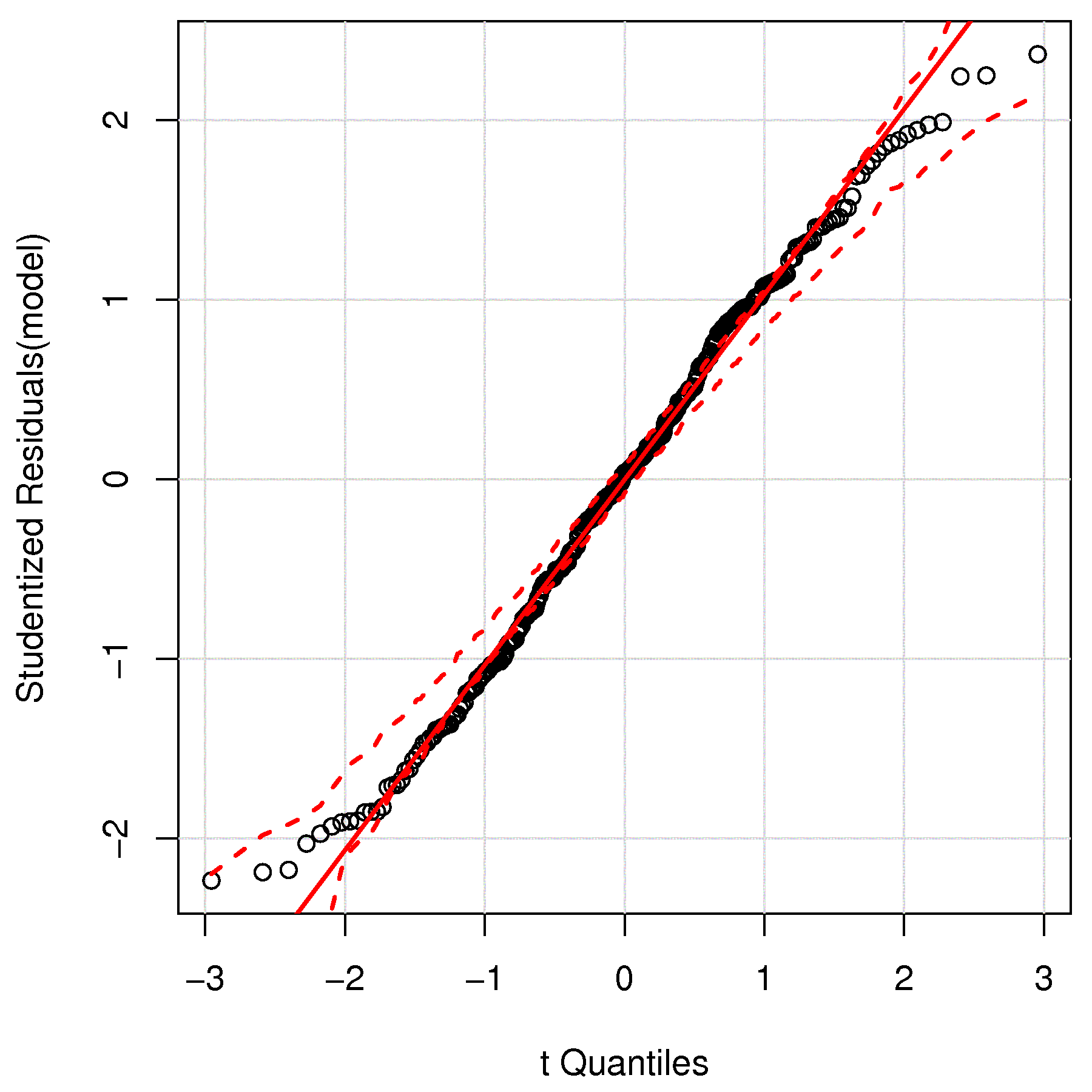
3. Are the residuals from the multiple linear regression model normally distributed?

4. In this part we are investigating the variance-covariance matrices used to calculate the linear model.

   1. First center the \(x\)-variables and the \(y\)-variable that you used in the model.

      Note: feel free to use MATLAB, or any other tool to answer this question. If you are using R, then you will benefit from this page in the R tutorial. Also, read the help for the model.matrix(...) function to get the \(\mathbf{X}\)-matrix. Then read the help for the sweep(...) function, or more simply use the scale(...) function to do the mean-centering.

   2. Show your calculated \(\mathbf{X}^T\mathbf{X}\) and \(\mathbf{X}^T\mathbf{y}\) variance-covariance matrices from the centered data.

   3. Explain why the interpretation of covariances in \(\mathbf{X}^T\mathbf{y}\) match the results from the full MLR model you calculated in part 1 of this question.

   4. Calculate \(\mathbf{b} =\left(\mathbf{X}^T\mathbf{X}\right)^{-1}\mathbf{X}^T\mathbf{y}\) and show that it agrees with the estimates that R calculated (even though R fits an intercept term, while your \(\mathbf{b}\) does not).

5. What would be the predicted yield for an experiment run without baffles, at 4000 rpm impeller speed, run at a reactor temperature of 90 °C?

Question 16

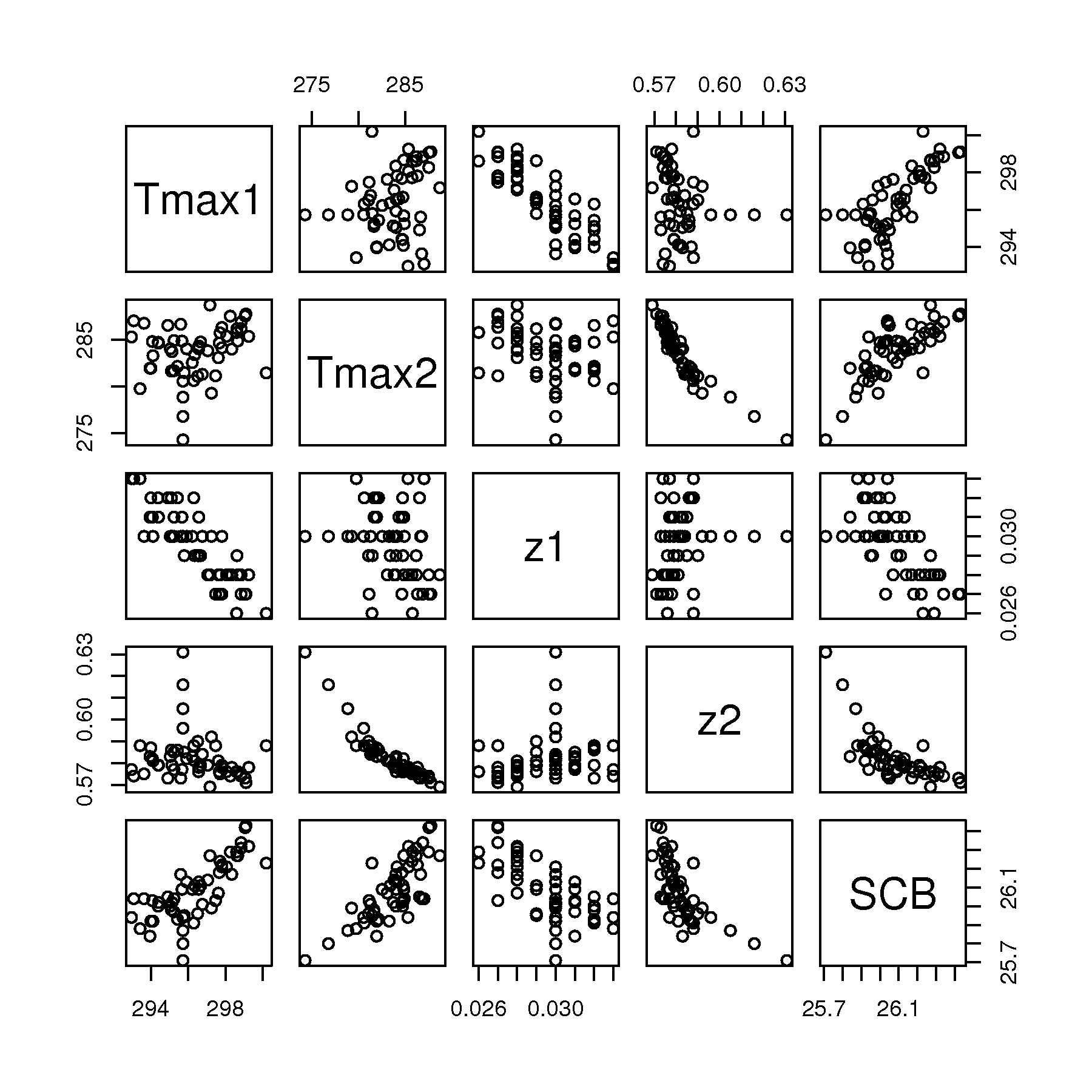
In this question we will use the LDPE data which is data from a high-fidelity simulation of a low-density polyethylene reactor. LDPE reactors are very long, thin tubes. In this particular case the tube is divided in 2 zones, since the feed enters at the start of the tube, and some point further down the tube (start of the second zone). There is a temperature profile along the tube, with a certain maximum temperature somewhere along the length. The maximum temperature in zone 1, Tmax1 is reached some fraction z1 along the length; similarly in zone 2 with the Tmax2 and z2 variables.

We will build a linear model to predict the SCB variable, the short chain branching (per 1000 carbon atoms) which is an important quality variable for this product. Note that the last 4 rows of data are known to be from abnormal process operation, when the process started to experience a problem. However, we will pretend we didn’t know that when building the model, so keep them in for now.

1. Use only the following subset of \(x\)-variables: Tmax1, Tmax2, z1 and z2 and the \(y\) variable = SCB. Show the relationship between these 5 variables in a scatter plot matrix.

   Use this code to get you started (make sure you understand what it is doing):

   LDPE <- read.csv('http://openmv.net/file/ldpe.csv')
   subdata <- data.frame(cbind(LDPE$Tmax1, LDPE$Tmax2, LDPE$z1, LDPE$z2, LDPE$SCB))
   colnames(subdata) <- c("Tmax1", "Tmax2", "z1", "z2", "SCB")
   

   Using bullet points, describe the nature of relationships between the 5 variables, and particularly the relationship to the \(y\)-variable.

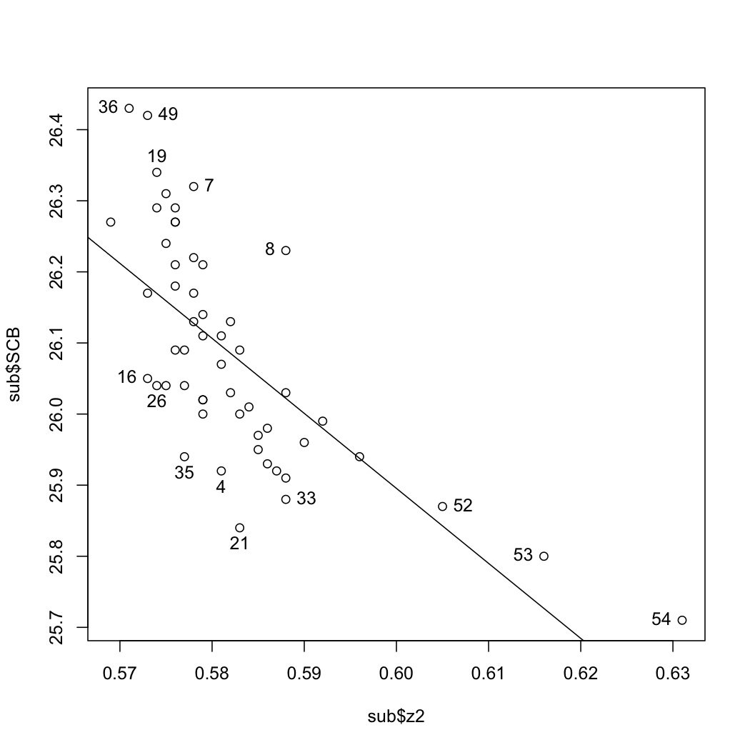
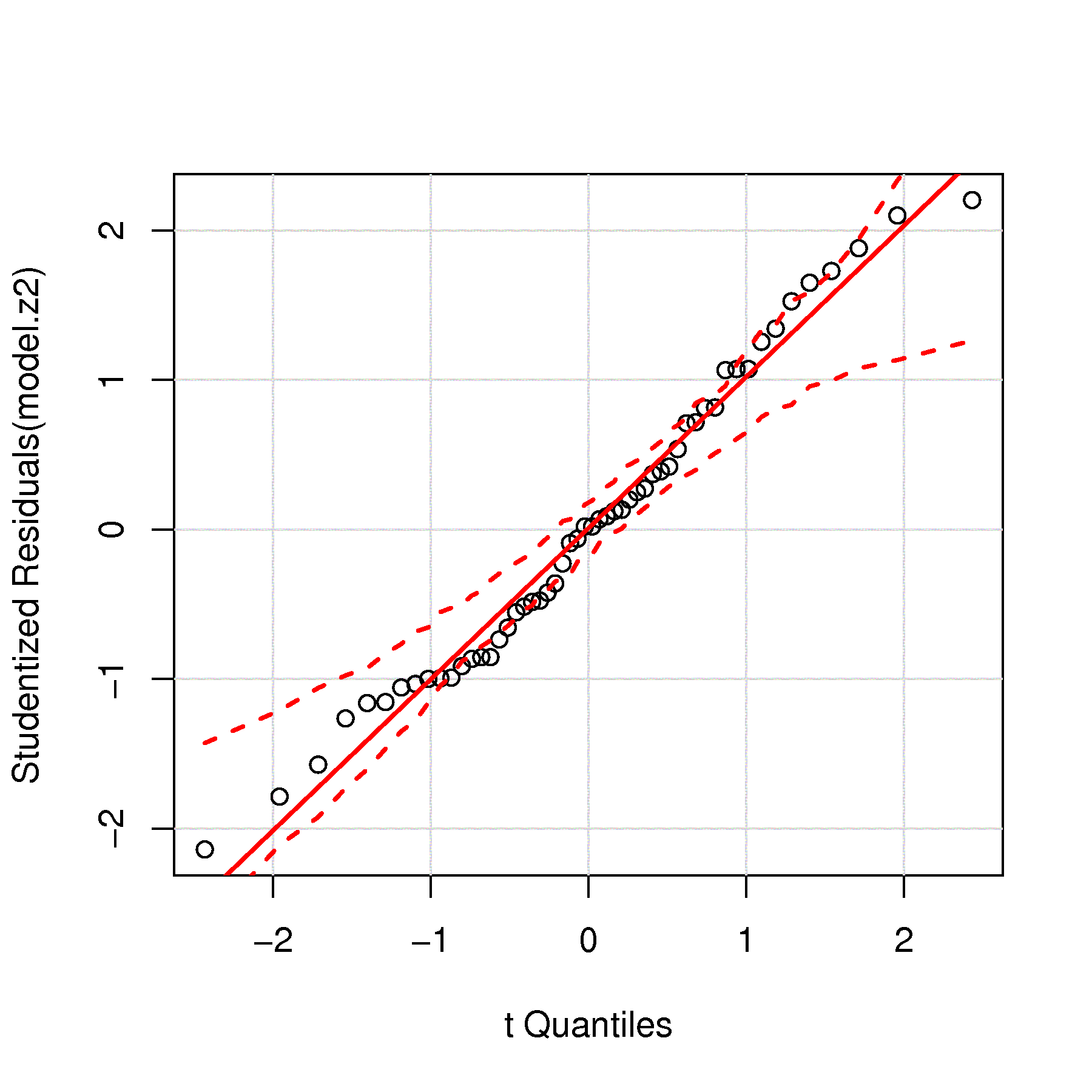
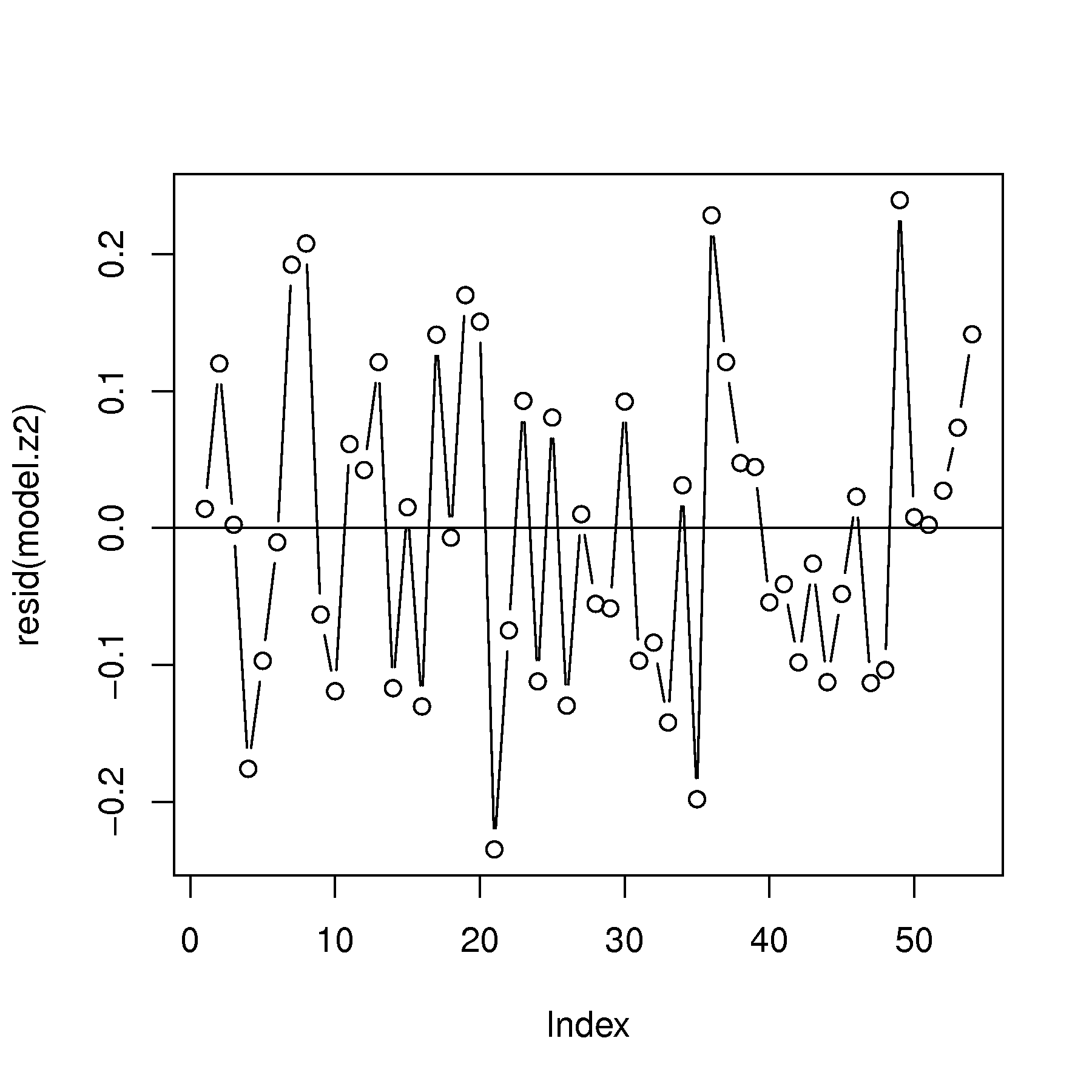
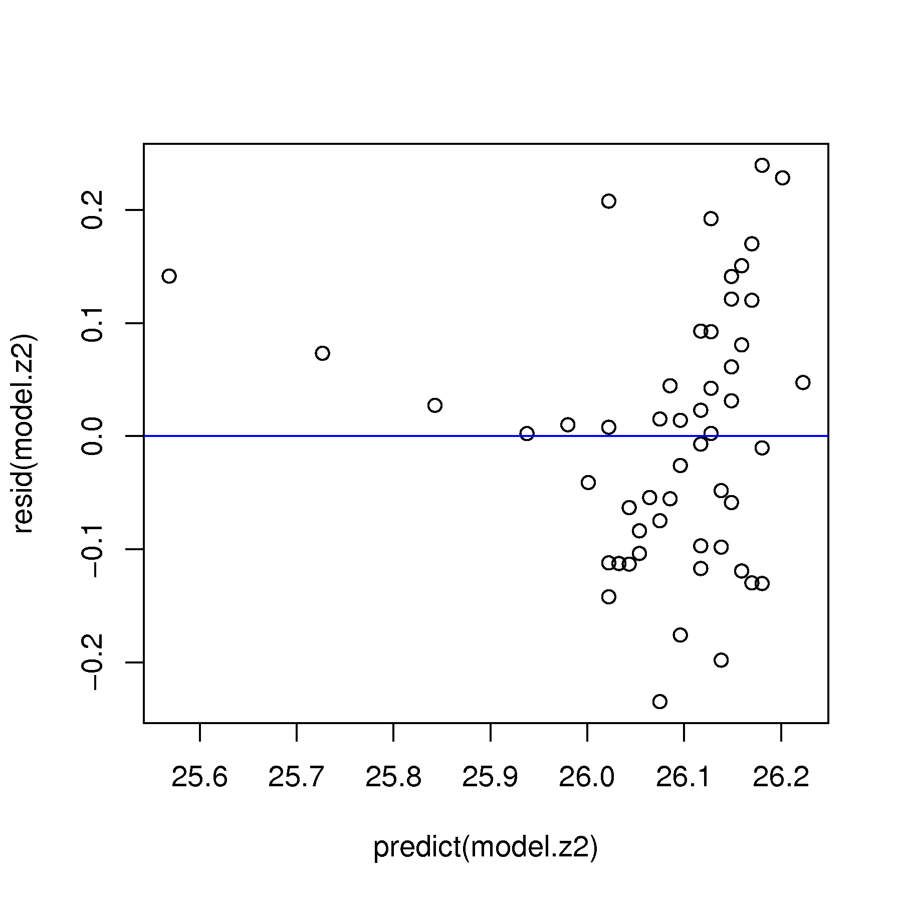
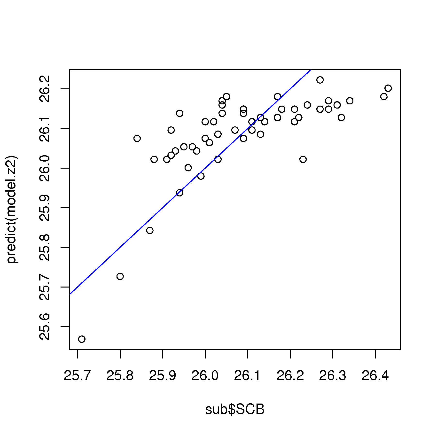
2. Let’s start with a linear model between z2 and SCB. We will call this the z2 model. Let’s examine its residuals:

   1. Are the residuals normally distributed?

   2. What is the standard error of this model?

   3. Are there any time-based trends in the residuals (the rows in the data are already in time-order)?

   4. Use any other relevant plots of the predicted values, the residuals, the \(x\)-variable, as described in class, and diagnose the problem with this linear model.

   5. What can be done to fix the problem? (You don’t need to implement the fix yet).

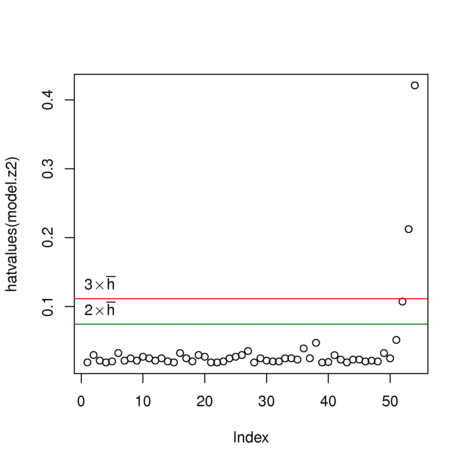
3. Show a plot of the hat-values (leverage) from the z2 model.

   1. Add suitable horizontal cut-off lines to your hat-value plot.

   2. Identify on your plot the observations that have large leverage on the model

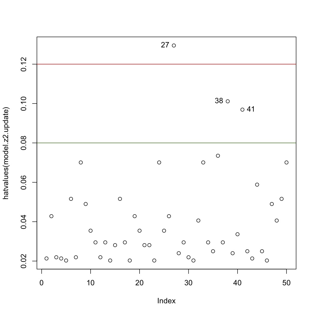
   3. Remove the high-leverage outliers and refit the model. Call this the z2.updated model

   4. Show the updated hat-values and verify whether the problem has mostly gone away

   Note: see the R tutorial on how to rebuild a model by removing points

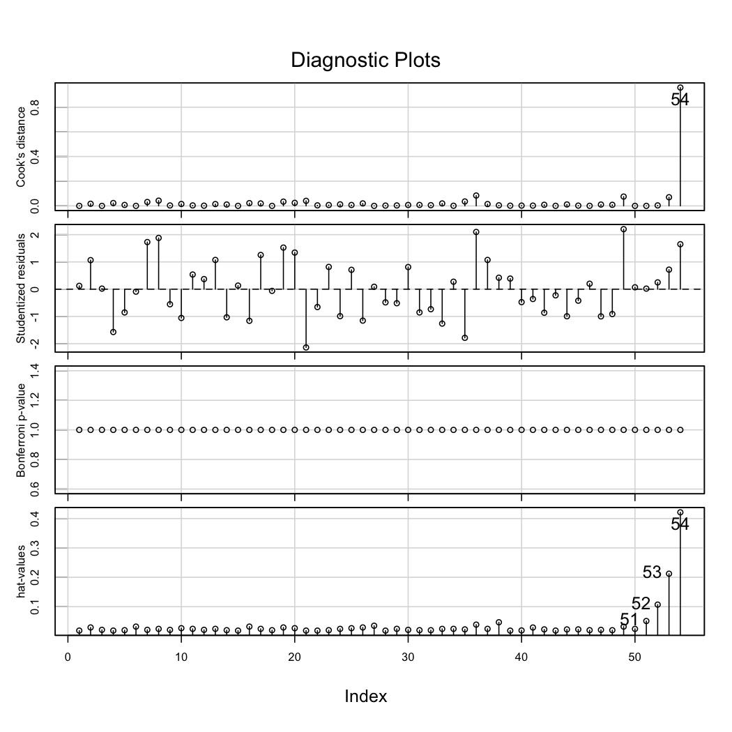
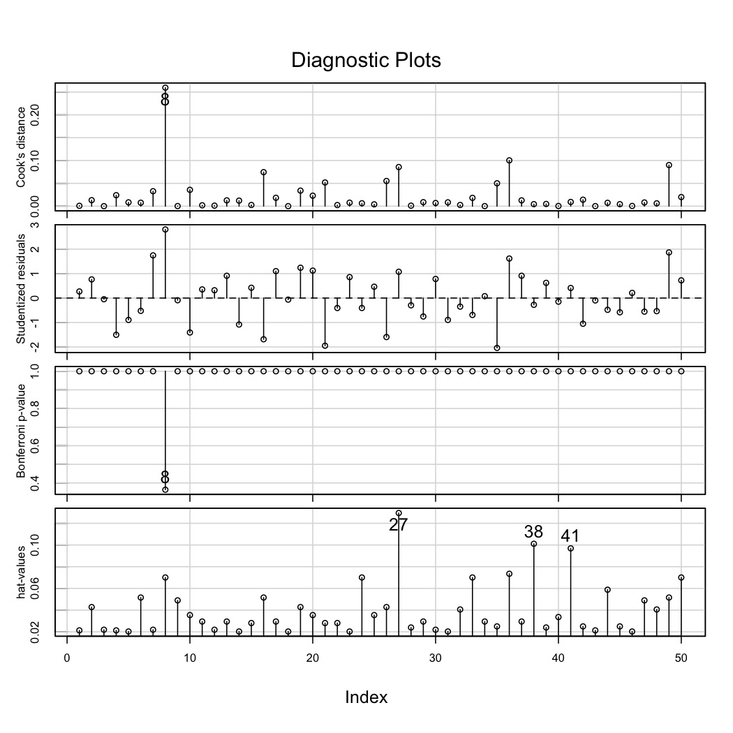
4. Use the influenceIndexPlot(...) function in the car library on both the z2 model and the z2.updated model. Interpret what each plot is showing for the two models. You may ignore the Bonferroni p-values subplot.

Solution Click to show answer

1. A scatter plot matrix of the 5 variables is

   

   • Tmax1 and z1 show a strongish negative correlation

   • Tmax1 and SCB show a strong positive correlation

   • Tmax2 and z2 have a really strong negative correlation, and the 4 outliers are very clearly revealed in almost any plot with z2

   • z1 and SCB have a negative correlation

   • Tmax2 and SCB have a negative correlation

   • Very little relationship appears between Tmax1 and Tmax2, which is expected, given how/where these 2 data variables are recorded.

   • Similarly for Tmax2 and z2.

2. A linear model between z2 and SCB: \(\widehat{\text{SCB}} = 32.23 - 10.6 z_2\)

   First start with a plot of the raw data with this regression line superimposed:

   

   which helps when we look at the q-q plot of the Studentized residuals to see the positive and the negative residuals:

   

   1. We notice there is no strong evidence of non-normality, however, we can see a trend in the tails on both sides (there are large positive residuals and large negative residuals). The identified points in the two plots help understand which points affect the residual tails.

   2. This model’s standard error is \(S_E = 0.114\), which should be compared to the range of the \(y\)-axis, 0.70 units, to get an idea whether this is large or small, so about 15% of the range. Given that a conservative estimate of the prediction interval is \(\pm 2 S_E\), or a total range of \(4S_E\), this is quite large.

   3. The residuals in time-order

      

      Show no consistent structure, however we do see the short upward trend in the last 4 points. The autocorrelation function (not shown here), shows there is no autocorrelation, i.e. the residuals appear independent.

   4. Three plots that do show a problem with the linear model:

      • Predictions vs residuals: definite structure in the residuals. We expect to see no structure, but a definite trend, formed by the 4 points is noticeable, as well as a negative correlation at high predicted SCB.

        

      • \(x\)-variable vs residuals: definite structure in the residuals, which is similar to the above plot.

      • Predicted vs measured \(y\): we expect to see a strong trend about a 45° line (shown in blue). The strong departure from this line indicates there is a problem with the model

        

   5. We can consider removing the 4 points that strongly bias the observed vs predicted plot above.

3. A plot of the hat-values (leverage) from the regression of SCB on z2 is:

   

   with 2 and 3 times the average hat value shown for reference. Points 52, 53 and 54 have leverage that is excessive, confirming what we saw in the previous part of this question.

   Once these points are removed, the model was rebuilt, and this time showed point 51 as an high-leverage outlier. This point was removed and the model rebuilt.

   The hat values from this updated model are:

   

   which is reasonable to stop at, since the problem has mostly gone away. If you keep omitting points, you will likely deplete all the data. At some point, especially when there is no obvious structure in the residuals, it is time to stop interrogating (i.e. investigating) and removing outliers.

   The updated model has a slightly improved standard error \(S_E = 0.11\) and the least squares model fit (see the R code) appears much more reasonable in the data.

4. The influence index plots for the model with all 54 points is shown first, followed by the influence index plot of the model with only the first 50 points.

   

   The increasing leverage, as the abnormal process operation develops is clearly apparent. This leverage is not “bad” (i.e. influential) initially, because it is “in-line” with the regression slope. But by observation 54, there is significant deviation that observation 54 has high residuals distance, and therefore a combined high influence on the model (high Cook’s D).

   

   The updated model shows shows only point 8 as an influential observation, due to its moderate leverage and large residual. However, this point does not warrant removal, since it is just above the cut-off value of \(4/(n-k) = 4/(50-2) = 0.083\) for Cook’s distance.

   The other large hat values don’t have large Studentized residuals, so they are not influential on the model.

   Notice how the residuals in the updated model are all a little smaller than in the initial model.

All the code for this question is given here:

LDPE <- read.csv('http://openmv.net/file/LDPE.csv')
summary(LDPE)
N <- nrow(LDPE)

sub <- data.frame(cbind(LDPE$Tmax1, LDPE$Tmax2, LDPE$z1, LDPE$z2, LDPE$SCB))
colnames(sub) <- c("Tmax1", "Tmax2", "z1", "z2", "SCB")

bitmap('ldpe-scatterplot-matrix.png', type="png256",
        width=6, height=6, res=300, pointsize=14)
plot(sub)
dev.off()

model.z2 <- lm(sub$SCB ~ sub$z2)
summary(model.z2)

# Plot raw data
bitmap('ldpe-z2-SCB-raw-data.png', type="png256",
        width=6, height=6, res=300, pointsize=14)
plot(sub$z2, sub$SCB)
abline(model.z2)
identify(sub$z2, sub$SCB)
dev.off()

# Residuals normal? Yes, but have heavy tails
bitmap('ldpe-z2-SCB-resids-qqplot.png', type="png256",
        width=6, height=6, res=300, pointsize=14)
library(car)
qqPlot(model.z2, id.method="identify")
dev.off()

# Residual plots in time order: no problems detected
# Also plotted the acf(...): no problems there either
bitmap('ldpe-z2-SCB-raw-resids-in-order.png', type="png256",
        width=6, height=6, res=300, pointsize=14)
plot(resid(model.z2), type='b')
abline(h=0)
dev.off()

acf(resid(model.z2))

# Predictions vs residuals: definite structure in the residuals!
bitmap('ldpe-z2-SCB-predictions-vs-residuals.png', type="png256",
        width=6, height=6, res=300, pointsize=14)        
plot(predict(model.z2), resid(model.z2))
abline(h=0, col="blue")
dev.off()
 
# x-data vs residuals: definite structure in the residuals!
bitmap('ldpe-z2-SCB-residual-structure.png', type="png256",
        width=6, height=6, res=300, pointsize=14)
plot(sub$Tmax2, resid(model.z2))
abline(h=0, col="blue")
identify(sub$z2, resid(model.z2))
dev.off()

# Predictions-vs-y
bitmap('ldpe-z2-SCB-predictions-vs-actual.png', type="png256",
        width=6, height=6, res=300, pointsize=14)
plot(sub$SCB, predict(model.z2))
abline(a=0, b=1, col="blue")
identify(sub$SCB, predict(model.z2))
dev.off()

# Plot hatvalues
bitmap('ldpe-z2-SCB-hat-values.png', type="png256",
        width=6, height=6, res=300, pointsize=14)
plot(hatvalues(model.z2))
avg.hat <- 2/N
abline(h=2*avg.hat, col="darkgreen")
abline(h=3*avg.hat, col="red")
text(3, y=2*avg.hat, expression(2 %*% bar(h)), pos=3)
text(3, y=3*avg.hat, expression(3 %*% bar(h)), pos=3)
identify(hatvalues(model.z2))
dev.off()

# Remove observations (observation 51 was actually detected after
# the first iteration of removing 52, 53, and 54: high-leverage points)
build <- seq(1,N)
remove <- -c(51, 52, 53, 54)
model.z2.update <- lm(model.z2, subset=build[remove])

# Plot updated hatvalues
plot(hatvalues(model.z2.update))
N <- length(model.z2.update$residuals)
avg.hat <- 2/N
abline(h=2*avg.hat, col="darkgreen")
abline(h=3*avg.hat, col="red")
identify(hatvalues(model.z2.update))
# Observation 27 still has high leverage: but only 1 point

# Problem in the residuals gone? Yes
plot(predict(model.z2.update), resid(model.z2.update))
abline(h=0, col="blue")

# Does the least squares line fit the data better?
plot(sub$z2, sub$SCB)
abline(model.z2.update)

# Finally, show an influence plot
influencePlot(model.z2, id.method="identify")
influencePlot(model.z2.update, id.method="identify")

# Or the influence index plots
influenceIndexPlot(model.z2, id.method="identify")
influenceIndexPlot(model.z2.update, id.method="identify")


#-------- Use all variables in an MLR (not required for question)

model.all <- lm(sub$SCB ~ sub$z1 + sub$z2 + sub$Tmax1 + sub$Tmax2)
summary(model.all)
confint(model.all)

Question 17

A concrete slump test is used to test for the fluidity, or workability, of concrete. It’s a crude, but quick test often used to measure the effect of polymer additives that are mixed with the concrete to improve workability.

The concrete mixture is prepared with a polymer additive. The mixture is placed in a mold and filled to the top. The mold is inverted and removed. The height of the mold minus the height of the remaining concrete pile is called the “slump”.

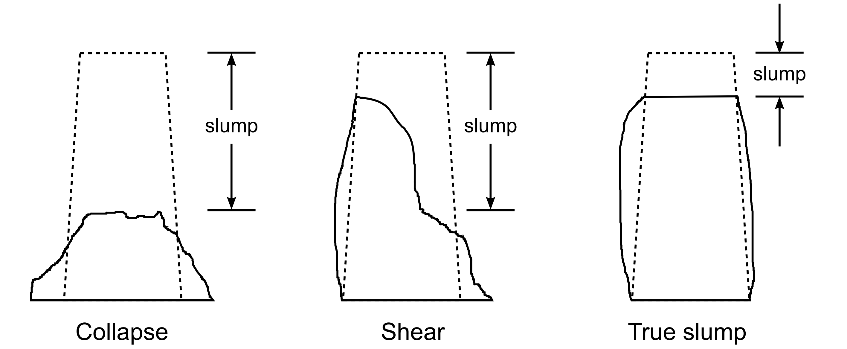
Figure from Wikipedia

Your company provides the polymer additive, and you are developing an improved polymer formulation, call it B, that hopefully provides the same slump values as your existing polymer, call it A. Formulation B costs less money than A, but you don’t want to upset, or lose, customers by varying the slump value too much.

The following slump values were recorded over the course of the day:

Additive	Slump value [cm]
A	5.2
A	3.3
B	5.8
A	4.6
B	6.3
A	5.8
A	4.1
B	6.0
B	5.5
B	4.5

You can derive the 95% confidence interval for the true, but unknown, difference between the effect of the two additives:

\[\begin{split}\begin{array}{rcccl} -c_t &\leq& z &\leq & +c_t \\ (\overline{x}_B - \overline{x}_A) - c_t \sqrt{s_P^2 \left(\frac{1}{n_B} + \frac{1}{n_A}\right)} &\leq& \mu_B - \mu_A &\leq & (\overline{x}_B - \overline{x}_A) + c_t \sqrt{s_P^2 \left(\frac{1}{n_B} + \frac{1}{n_A}\right)}\\ 1.02 - 2.3 \sqrt{0.709 \left(\frac{1}{5} + \frac{1}{5}\right)} &\leq& \mu_B - \mu_A &\leq& 1.02 + 2.3 \sqrt{0.709 \left(\frac{1}{5} + \frac{1}{5}\right)} \\ -0.21 &\leq& \mu_B - \mu_A &\leq& 2.2 \end{array}\end{split}\]

Fit a least squares model to the data using an integer variable, \(x_A = 0\) for additive A, and \(x_A = 1\) for additive B. The model should include an intercept term also: \(y = b_0 + b_A x_A\). Hint: use R to build the model, and search the R tutorial with the term categorical variable or integer variable for assistance.

Show that the 95% confidence interval for \(b_A\) gives exactly the same lower and upper bounds, as derived above with the traditional approach for tests of differences.

Solution Click to show answer

This short piece of R code shows the expected result when regressing the slump value onto the binary factor variable:

additive <- as.factor(c("A", "A", "B", "A", "B", "A", "A", "B", "B", "B"))
slump <- c(5.2, 3.3, 5.8, 4.6, 6.3, 5.8, 4.1, 6.0, 5.5, 4.5)
confint(lm(slump ~ additive))

                 2.5 %   97.5 %
(Intercept)  3.7334823 5.466518
additive    -0.2054411 2.245441

Note that this approach works only if your coding has a one unit difference between the two levels. For example, you can code \(A = 17\) and \(B = 18\) and still get the same result. Usually though \(A=0\) and \(B=1\) or the \(A = 1\) and \(B = 2\) coding is the most natural, but all 3 of these codings would give the same confidence interval (the intercept changes though).

Question 18

Some data were collected from tests where the compressive strength, \(x\), used to form concrete was measured, as well as the intrinsic permeability of the product, \(y\). There were 16 data points collected. The mean \(x\)-value was \(\overline{x} = 3.1\) and the variance of the \(x\)-values was 1.52. The average \(y\)-value was 40.9. The estimated covariance between \(x\) and \(y\) was \(-5.5\).

The least squares estimate of the slope and intercept was: \(y = 52.1 - 3.6 x\).

1. What is the expected permeability when the compressive strength is at 5.8 units?

2. Calculate the 95% confidence interval for the slope if the standard error from the model was 4.5 units. Is the slope coefficient statistically significant?

3. Provide a rough estimate of the 95% prediction interval when the compressive strength is at 5.8 units (same level as for part 1). What assumptions did you make to provide this estimate?

4. Now provide a more accurate, calculated 95% prediction confidence interval for the previous part.

Question 19

A simple linear model relating reactor temperature to polymer viscosity is desirable, because measuring viscosity online, in real time is far too costly, and inaccurate. Temperature, on the other hand, is quick and inexpensive. This is the concept of soft sensors, also known as inferential sensors.

Data were collected from a rented online viscosity unit and a least squares model build:

\[\hat{v} = 1977 - 3.75 T\]

where the viscosity, \(v\), is measured in Pa.s (Pascal seconds) and the temperature is in Kelvin. A reasonably linear trend was observed over the 86 data points collected. Temperature values were taken over the range of normal operation: 430 to 480 K and the raw temperature data had a sample standard deviation of 8.2 K.

The output from a certain commercial software package was:

                    Analysis of Variance
---------------------------------------------------------
                                    Sum of           Mean
Source                   DF        Squares         Square
Model                     2         9532.7        4766.35
Error                    84         9963.7          118.6
Total                    86        19496.4
Root MSE              XXXXX
R-Square              XXXXX

1. Which is the causal direction: does a change in viscosity cause a change in temperature, or does a change in temperature cause a change in viscosity?

2. Calculate the Root MSE, what we have called standard error, \(S_E\) in this course.

3. What is the \(R^2\) value that would have been reported in the above output?

4. What is the interpretation of the slope coefficient, -3.75, and what are its units?

5. What is the viscosity prediction at 430K? And at 480K?

6. In the future you plan to use this model to adjust temperature, in order to meet a certain viscosity target. To do that you must be sure the change in temperature will lead to the desired change in viscosity.

   What is the 95% confidence interval for the slope coefficient, and interpret this confidence interval in the context of how you plan to use this model.

7. The standard error features prominently in all derivations related to least squares. Provide an interpretation of it and be specific in any assumption(s) you require to make this interpretation.

Solution Click to show answer

1. The causal direction is that a change in temperature causes a change in viscosity.

2. The Root MSE \(= S_E = \displaystyle \sqrt{\frac{\sum{e_i^2}}{n-k}} = \sqrt{\frac{\displaystyle 9963.7}{84}} = \bf{10.9}\) Pa.s.

3. \(R^2 = \displaystyle \frac{\text{RegSS}}{\text{TSS}} = \frac{9532.7}{19496.4} = \bf{0.49}\)

4. The slope coefficient is \(-3.75 \frac{\text{Pa.s}}{\text{}K}\) and implies that the viscosity is expected to decrease by 3.75 Pa.s for every one degree increase in temperature.

5. The viscosity prediction at 430K is \(1977 - 3.75 \times 430 = \bf{364.5}\) Pa.s and is \(\bf{177}\) Pa.s at 480 K.

6. The confidence interval is

   \[\begin{split}b_1 & \pm c_t S_E(b_1)\\ -3.75 & \pm 1.98\displaystyle \frac{S_E^2}{\sum_{j}{\left(x_j - \overline{x}\right)^2}} \\ -3.75 & \pm 1.98\frac{10.9}{697}\\ -3.75 & \pm 0.031\end{split}\]

   where \(\displaystyle \frac{\left(x_j - \overline{x}\right)^2}{n-1} = 8.2\), so one can solve for \(\displaystyle \left(x_j - \overline{x}\right)^2\) (though any reasonable value/attempt to get this value should be acceptable) and \(c_t = 1.98\), using \(n-k\) degrees of freedom at 95% confidence.

   Interpretation: this interval is extremely narrow, i.e. our slope estimate is precise. We can be sure that any change made to the temperature in our system will have the desired effect on viscosity in the feedback control system.

7. The standard error, \(S_E = 10.9\) Pa.s is interpreted as the amount of spread in the residuals. In addition, if we assume the residuals to be normally distributed (easily confirmed with a q-q plot) and independent. If that is true, then \(S_E\) is the one-sigma standard deviation for the residuals and we can say 95% of the residuals are expected within a range of \(\pm 2 S_E\).