6.5.5. PCA example: Food texture analysis

Let’s take a look at an example to consolidate and extend the ideas introduced so far. This data set is from a food manufacturer making a pastry product. Each sample (row) in the data set is taken from a batch of product where 5 quality attributes are measured:

1. Percentage oil in the pastry

2. The product’s density (the higher the number, the more dense the product)

3. A crispiness measurement, on a scale from 7 to 15, with 15 being more crispy.

4. The product’s fracturability: the angle, in degrees, through which the pasty can be slowly bent before it fractures.

5. Hardness: a sharp point is used to measure the amount of force required before breakage occurs.

A scatter plot matrix of these \(K = 5\) measurements is shown for the \(N=50\) observations.

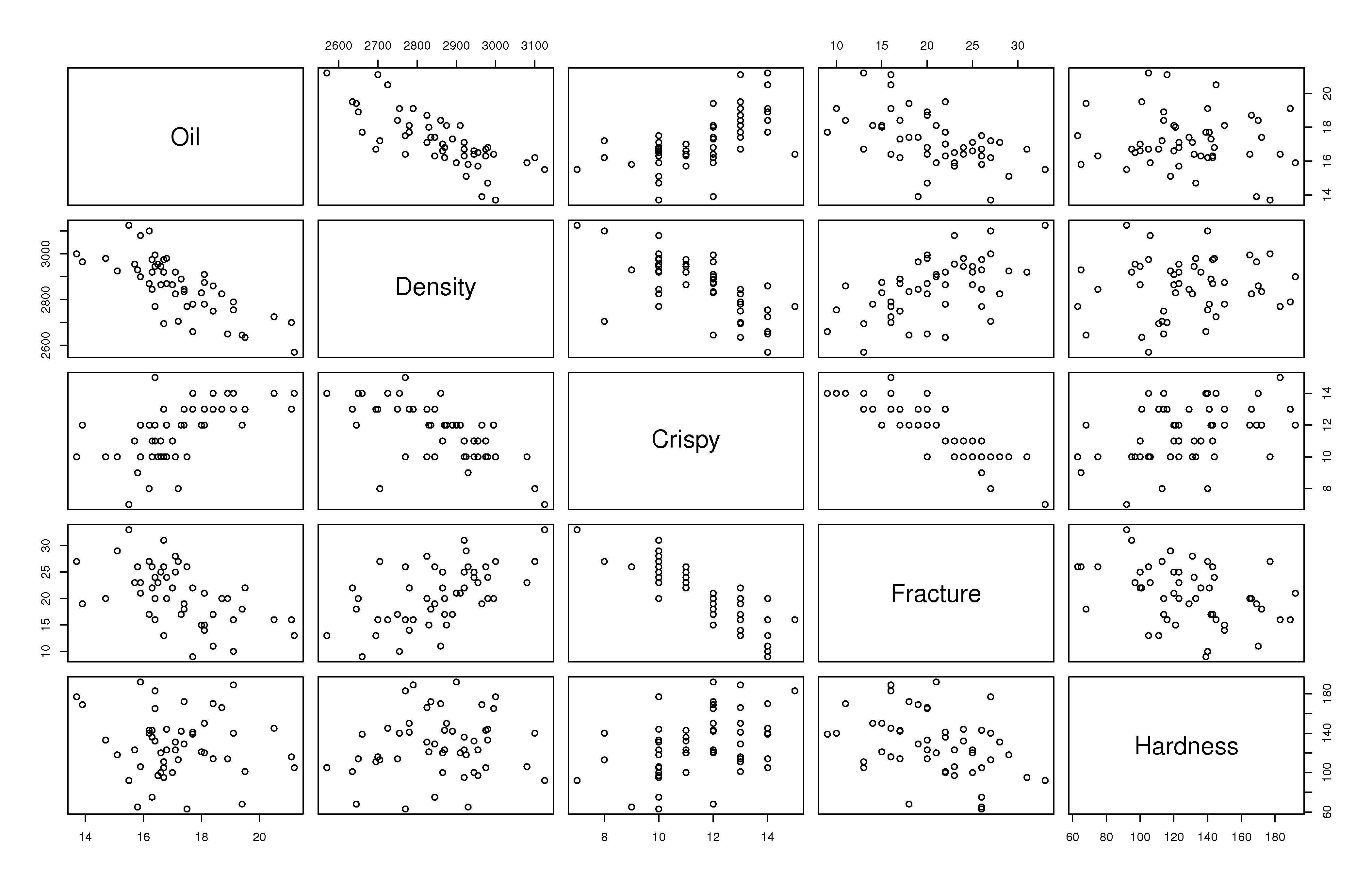
We can get by with this visualization of the data because \(K\) is small in this case. This is also a good starting example, because you can refer back to these scatterplots to confirm your findings.

Preprocessing the data

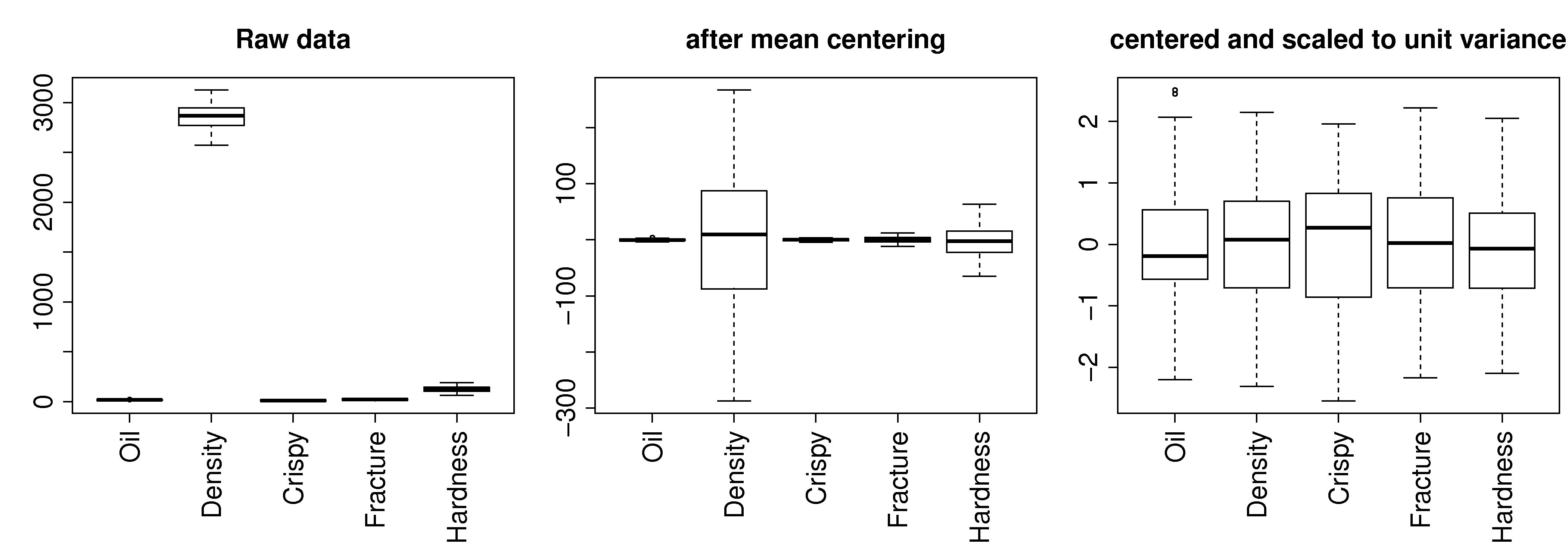
The first step with PCA is to center and scale the data. The box plots show how the raw data are located at different levels and have arbitrary units.

Centering removes any bias terms from the data by subtracting the mean value from each column in the matrix \(\mathbf{X}\). For the \(k^\text{th}\) column:

\[\mathbf{x}_{k,\text{center}} = \mathbf{x}_{k,\text{raw}} - \text{mean}\left(\mathbf{x}_{k,\text{raw}}\right)\]

Scaling removes the fact that the raw data could be in diverse units:

\[\mathbf{x}_{k} = \dfrac{\mathbf{x}_{k,\text{center}}}{ \text{standard deviation}\left(\mathbf{x}_{k,\text{center}}\right) }\]

Then each column \(\mathbf{x}_{k}\) is collected back to form matrix \(\mathbf{X}\). This preprocessing is so common it is called autoscaling: center each column to zero mean and then scale it to have unit variance. After this preprocessing each column will have a mean of 0.0 and a variance of 1.0. (Note the box plots don’t quite show this final result, because they use the median instead of the mean, and show the interquartile range instead of the standard deviation).

Centering and scaling does not alter the overall interpretation of the data: if two variables were strongly correlated before preprocessing they will still be strongly correlated after preprocessing.

For reference, the mean and standard deviation of each variable is recorded below. In the last 3 columns we show the raw data for observation 33, the raw data after centering, and the raw data after centering and scaling:

Variable	Mean	Standard deviation	Raw data	After centering	After autoscaling
Oil	17.2	1.59	15.5	-1.702	-1.069
Density	2857.6	124.5	3125	267.4	+2.148
Crispy	11.52	1.78	7	-4.52	-2.546
Fracture	20.86	5.47	33	12.14	+2.221
Hardness	128.18	31.13	92	-36.18	-1.162

Loadings: \(\,\mathbf{p}_1\)

We will discuss how to determine the number of components to use in a future section, and how to compute them, but for now we accept there are two important components, \(\mathbf{p}_1\) and \(\mathbf{p}_2\). They are:

\[\begin{split}\mathbf{p}_1 = \begin{bmatrix} +0.46 \\ -0.47 \\ +0.53 \\ -0.50 \\ +0.15 \end{bmatrix} \qquad \text{and} \qquad \mathbf{p}_2 = \begin{bmatrix} -0.37 \\ +0.36 \\ +0.20 \\ -0.22 \\ +0.80 \end{bmatrix}\\\end{split}\]

Where we might visualize that first component by a bar plot:

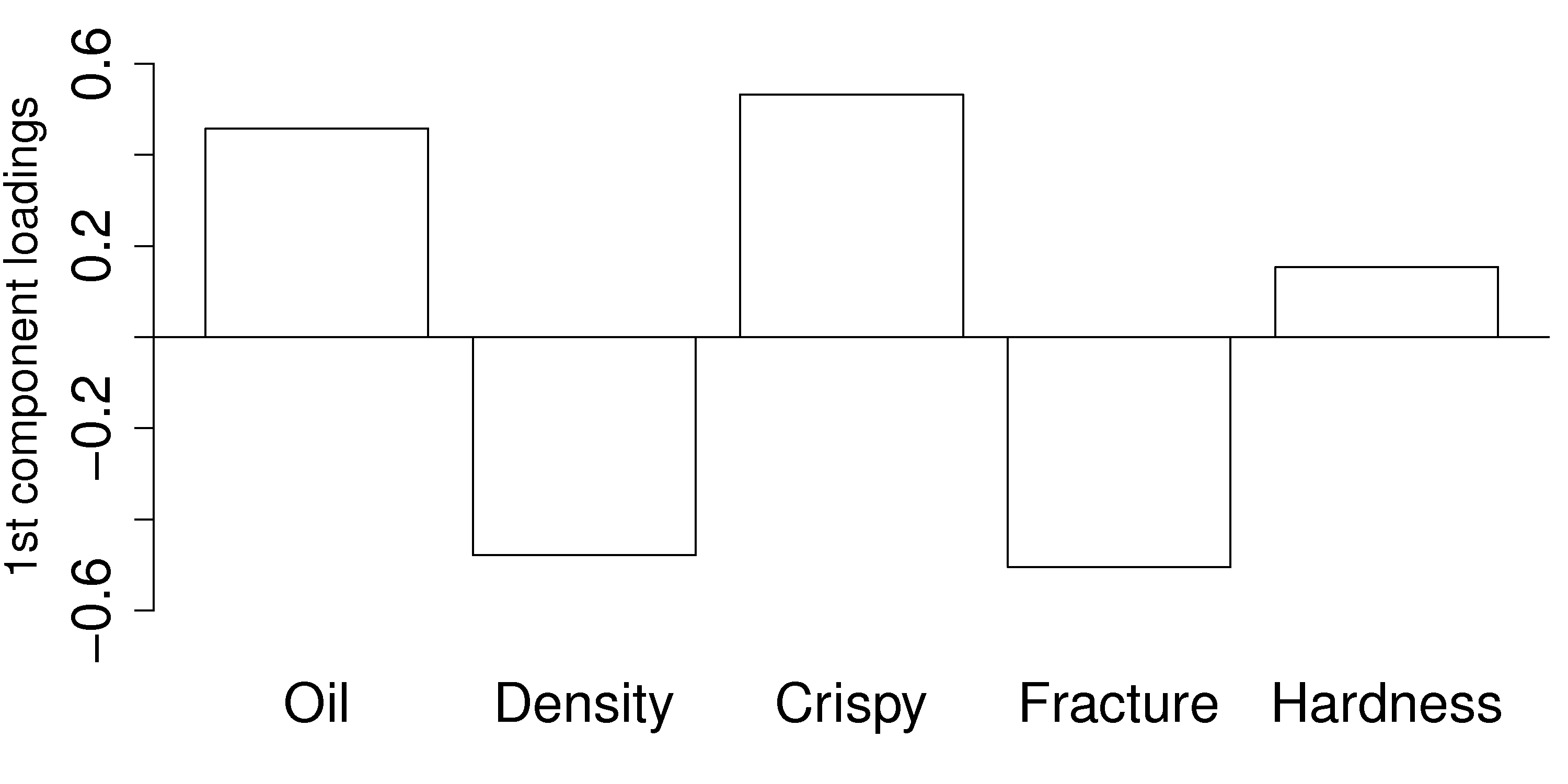
This plot shows the first component. All variables, except for hardness have large values in \(\mathbf{p}_1\). If we write out the equation for \(t_1\) for an observation \(i\):

(1)\[t_{i,1} = 0.46 \,\, x_\text{oil} - 0.47 \,\, x_\text{density} + 0.53 \,\, x_\text{crispy} - 0.50 \,\, x_\text{fracture} + 0.15 \,\, x_\text{hardness}\]

Once we have centered and scaled the data, remember that a negative \(x\)-value is a value below the average, and that a positive \(x\)-value lies above the average.

For a pastry product to have a high \(t_1\) value would require it to have some combination of above-average oil level, low density, and/or be more crispy and/or only have a small angle by which it can be bent before it fractures, i.e. low fracturability. So pastry observations with high \(t_1\) values sound like they are brittle, flaky and light. Conversely, a product with low \(t_1\) value would have the opposite sort of conditions: it would be a heavier, more chewy pastry (higher fracture angle) and less crispy.

Scores: \(\,\mathbf{t}_1\)

Let’s examine the score values calculated. As shown in equation (1), the score value is a linear combination of the data, \(\mathbf{x}\), given by the weights in the loadings matrix, \(\mathbf{P}\). For the first component, \(\mathbf{t}_1 = \mathbf{X} \mathbf{p}_1\). The plot here shows the values in vector \(\mathbf{t}_1\) (an \(N \times 1\) vector) as a sequence plot

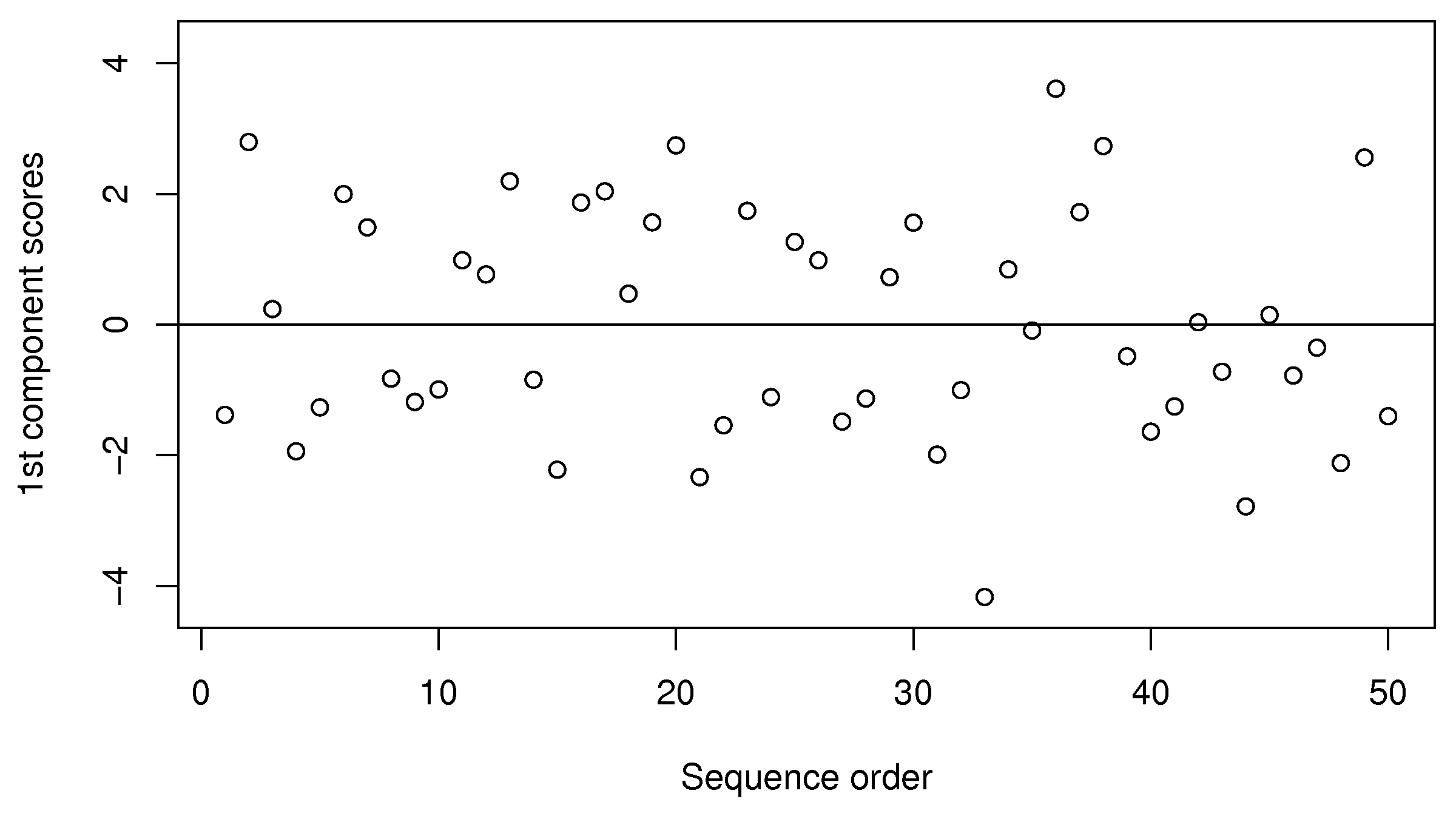
The samples appear to be evenly spread, some high and some low on the \(t_1\) scale. Sample 33 has a \(t_1\) value of -4.2, indicating it was much denser than the other pastries, and had a high fracture angle (it could be bent more than others). In fact, if we refer to the raw data we can confirm these findings: \(\mathbf{x}_{i=33} = [15.5, \,\, 3125, \,\, 7, \,\, 33, \,\, 92]\). Also refer back to the scatterplot matrix and mark the point which has density of 3125, and fracture angle of 33. This pastry also has a low oil percentage (15.5%) and low crispy value (7).

We can also investigate sample 36, with a \(t_1\) value of 3.6. The raw data again confirm that this pastry follows the trends of other, high \(t_1\) value pastries. It has a high oil level, low density, high crispiness, and a low fracture angle: \(x_{36} = [21.2, \,\, 2570, \,\, 14, \,\, 13, \,\, 105]\). Locate again on the scatterplot matrices sample 36 where oil level is 21.2 and the crispiness is 14. Also mark the point where density = 2570 and the fracture value = 13 for this sample.

We note here that this component explains 61% of the original variability in the data. It’s hard to say whether this is high or low, because we are unsure of the degree of error in the raw data, but the point is that a single variable summarizes about 60% of the variability from all 5 columns of raw data.

Loadings: \(\,\mathbf{p}_2\)

The second loading vector is shown as a bar plot:

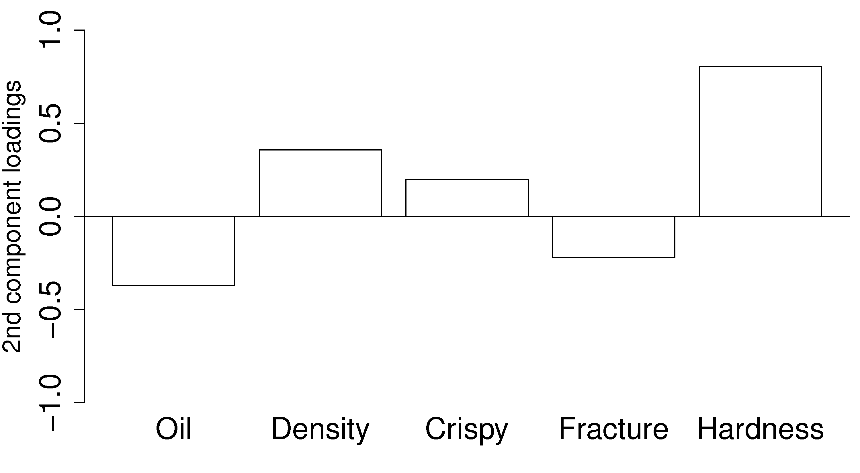
This direction is aligned mainly with the hardness variable: all other variables have a small coefficient in \(\mathbf{p}_2\). A high \(t_2\) value is straightforward to interpret: it would imply the pastry has a high value on the hardness scale. Also, this component explains an additional 26% of the variability in the dataset.

Because this component is orthogonal to the first component, we can be sure that this hardness variation is independent of the first component. One valuable way to interpret and use this information is that you can adjust the variables in \(\mathbf{p}_2\), i.e. the process conditions that affect the pastry’s hardness, without affecting the other pastry properties, i.e the variables described in \(\mathbf{p}_1\).