6.5.10. Interpreting the residuals

We consider three types of residuals: residuals within each row of \(\mathbf{X}\), called squared prediction errors (SPE); residuals for each column of \(\mathbf{X}\), called \(R^2_k\) for each column, and finally residuals for the entire matrix \(\mathbf{X}\), usually just called \(R^2\) for the model.

6.5.10.1. Residuals for each observation: the square prediction error

We have already introduced the squared prediction error geometrically. We showed in that section that the residual distance from the actual observation to the model plane is given by:

\[\begin{split}\mathbf{e}'_{i,A} &= \mathbf{x}'_i - \widehat{\mathbf{x}}'_{i,A} \\ \mathbf{e}'_{i,A} &= \mathbf{x}'_i - \mathbf{t}'_i \mathbf{P}'\end{split}\]

Turning this last equation around we have:

\[\begin{split}\mathbf{x}'_i &= \mathbf{t}'_i \mathbf{P}' + \mathbf{e}'_{i,A} \\ (1 \times K) &= (1 \times A)(A \times K) + (1 \times K)\end{split}\]

Or in general, for the whole data set

\[\begin{split}\mathbf{X} &= \mathbf{T} \mathbf{P}' + \mathbf{E} = \widehat{\mathbf{X}} + \mathbf{E} \\ (N \times K) &= (N \times A)(A \times K) + (N \times K)\end{split}\]

This shows that each observation (row in \(\mathbf{X}\)) can be split and interpreted in two portions: a vector on-the-plane, \(\mathbf{t}'_i \mathbf{P}'\), and a vector perpendicular to the plane, \(\mathbf{e}'_{i,A}\). This residual portion, a vector, can be reduced to a single number, a distance value called SPE, as previously described.

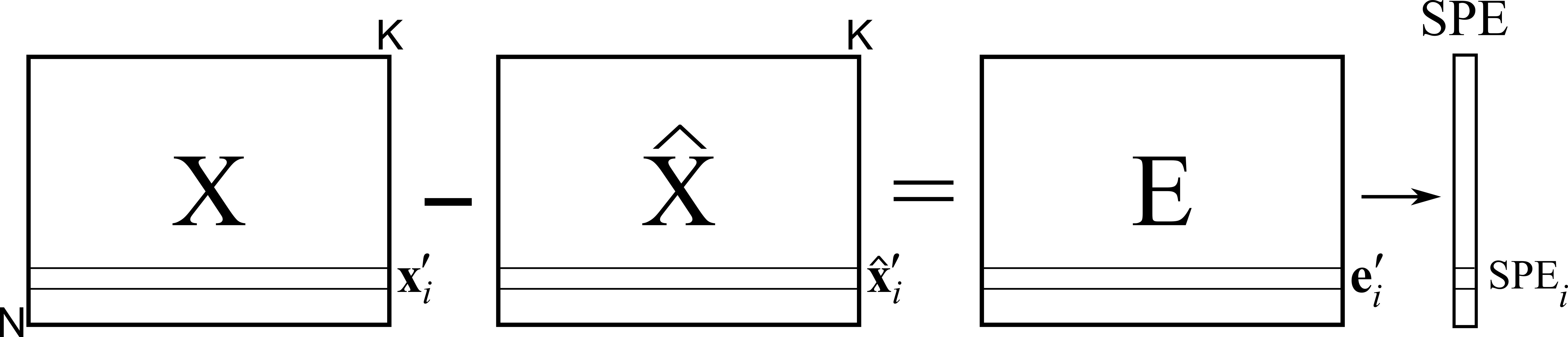
An observation in \(\mathbf{X}\) that has \(\text{SPE}_i = 0\) is exactly on the plane and follows the model structure exactly; this is the smallest SPE value possible. For a given data set we have a distribution of SPE values. We can calculate a confidence limit below which we expect to find a certain fraction of the data, e.g. a 95% confidence limit. We won’t go into how this limit is derived, suffice to say that most software packages will compute it and show it.

The most convenient way to visualize these SPE values is as a sequence plot, or a line plot, where the \(y\)-axis has a lower limit of 0.0, and the 95% and/or 99% SPE limit is also shown. Remember that we would expect 5 out of 100 points to naturally fall above the 95% limit.

If we find an observation that has a large squared prediction error, i.e. the observation is far off the model plane, then we say this observation is inconsistent with the model. For example, if you have data from a chemical process, taken over several days, your first 300 observations show SPE values below the limit. Then on the 4th day you notice a persistent trend upwards in SPE values: this indicates that those observations are inconsistent with the model, indicating a problem with the process, as reflected in the data captured during that time.

We would like to know why, specifically which variable(s) in \(\mathbf{X}\), are most related with this deviation off the model plane. As we did in the section on interpreting scores, we can generate a contribution plot.

\[\mathbf{e}'_{i,A} = \mathbf{x}'_i - \widehat{\mathbf{x}}'_{i,A}\]

Dropping the \(A\) subscript for convenience we can write the \(1 \times K\) vector as:

\[\begin{split}\mathbf{e}'_{i} &= \mathbf{x}'_i - \widehat{\mathbf{x}}'_{i} \\ (1 \times K) &= \begin{bmatrix}(x_{i,1} - \hat{x}_{i,1}) & (x_{i,2} - \hat{x}_{i,2}) & \ldots & (x_{i,k} - \hat{x}_{i,k}) & \ldots & (x_{i,K} - \hat{x}_{i,K})\end{bmatrix}\end{split}\]

The SPE is just the sum of the squares of these \(K\) terms, so a residual contribution plot, most conveniently shown as a bar chart of these \(K\) terms, indicates which of the original \(K\) variable(s) are most associated with the deviation off the model plane. We say that the correlation structure among these variables has been broken. This is because PCA provides a model of the correlation structure in the data table. When an observation has a large residual, then that observation is said to break the correlation structure, and is inconsistent with the model.

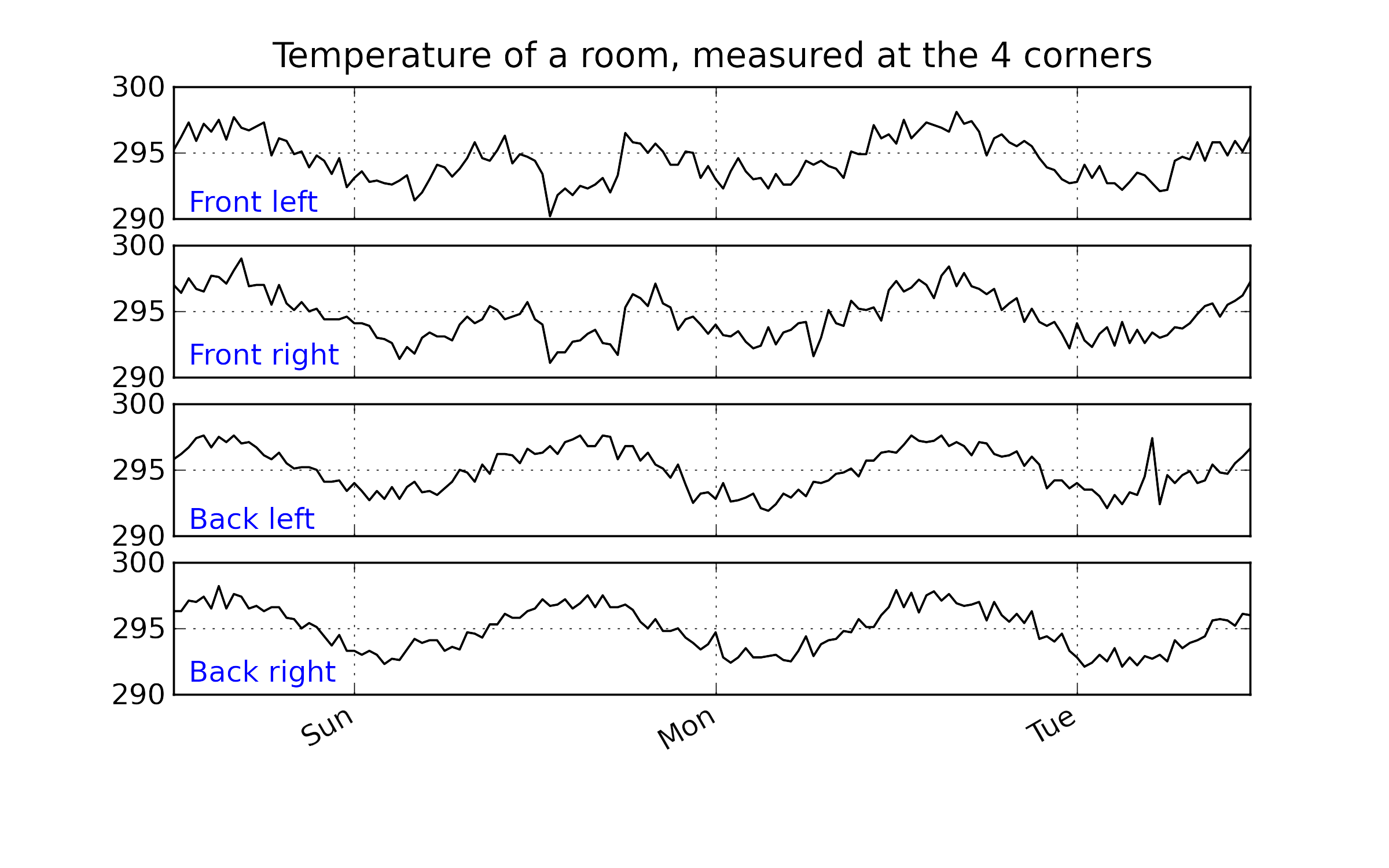
Looking back at the room-temperature example: if we fit a model with one component, then the residual distance, shown with the 95% limit, appears as follows:

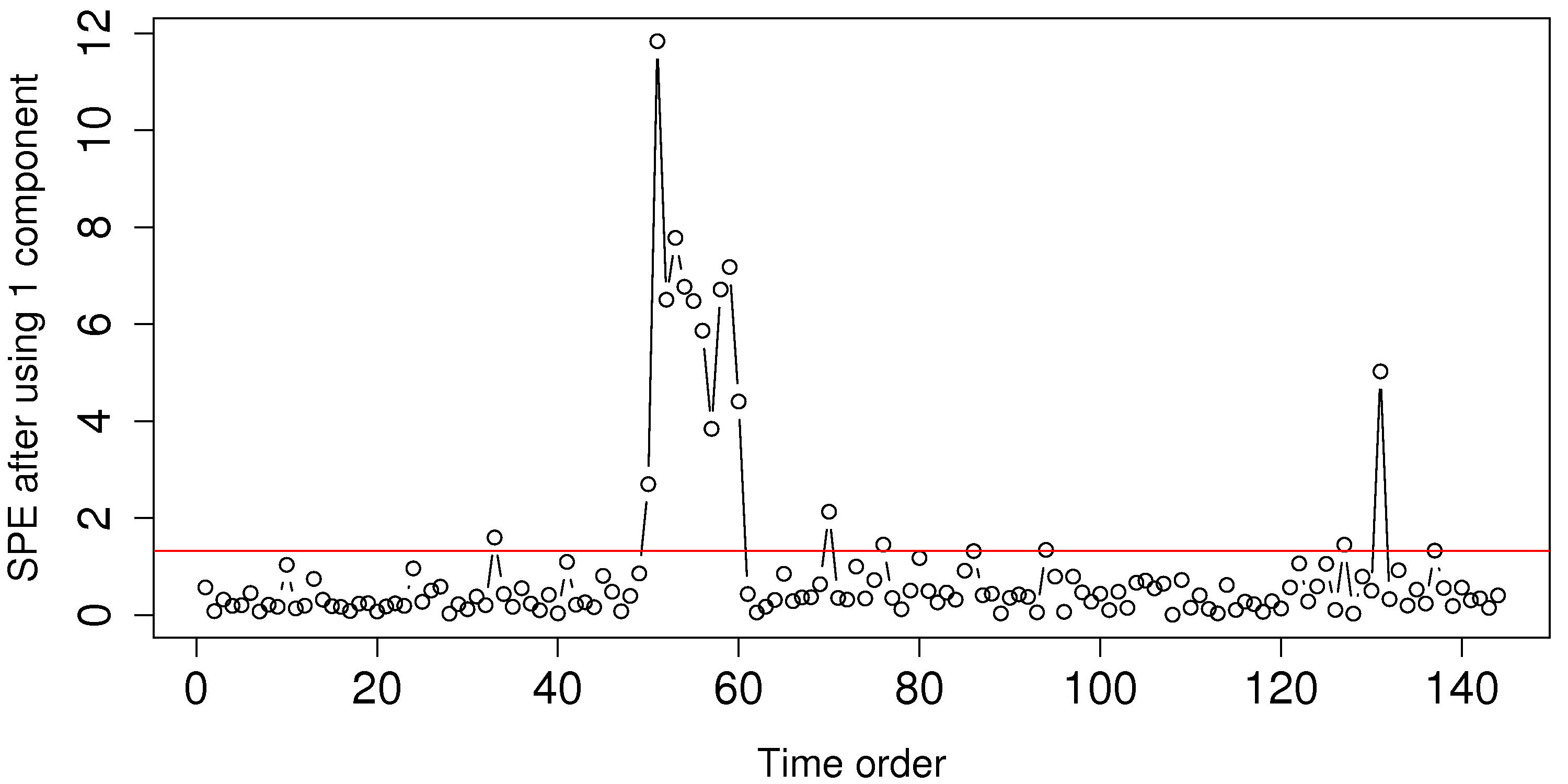
Using the raw data for this example, shown below, can you explain why we see those unusual points in the SPE plot around time 50 to 60?

Finally, the SPE value is a complete summary of the residual vector. As such, it is sometimes used to colour-code score plots, as we mentioned back in the section on score plots. Another interesting way people sometimes display SPE is to plot a 3D data cloud, with \(\mathbf{t}_1\) and \(\mathbf{t}_2\), and use the SPE values on the third axis. This gives a fairly complete picture of the major dimensions in the model: the explained variation on-the-plane, given by \(\mathbf{t}_1\) and \(\mathbf{t}_2\), and the residual distance off-the-plane, summarized by SPE.

6.5.10.2. Residuals for each column

Using the residual matrix \(\mathbf{E} = \mathbf{X} - \mathbf{T} \mathbf{P}' = \mathbf{X} - \widehat{\mathbf{X}}\), we can calculate the residuals for each column in the original matrix. This is summarized by the \(R^2\) value for each column in \(\mathbf{X}\) and gives an indication of how well the PCA model describes the data from that column.

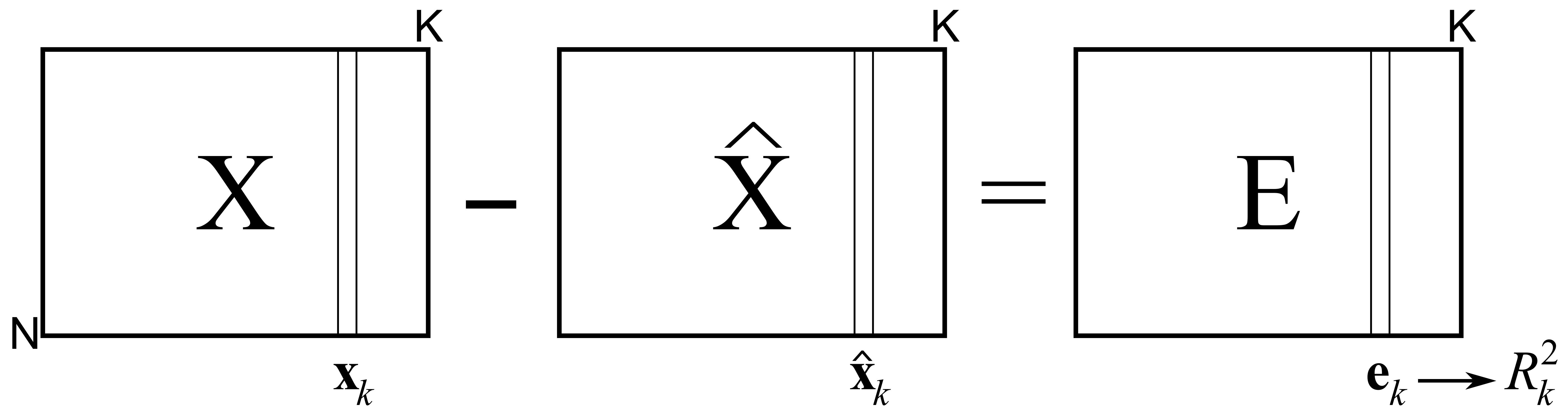
In the section on least squares modelling, the \(R^2\) number was shown to be the ratio between the variance remaining in the residuals over the total variances we started off with, subtracted from 1.0. Using the notation in the previous illustration:

\[R^2_k = 1 - \dfrac{\text{Var}(\mathbf{x}_k - \widehat{\mathbf{x}}_k)}{\text{Var}(\mathbf{x}_k)} = 1 - \dfrac{\text{Var}(\mathbf{e}_k)}{\text{Var}(\mathbf{x}_k)}\]

The \(R^2_k\) value for each variable will increase with every component that is added to the model. The minimum value is 0.0 when there are no components (since \(\widehat{\mathbf{x}}_k = \mathbf{0}\)), and the maximum value is 1.0, when the maximum number of components have been added (and \(\widehat{\mathbf{x}}_k = \mathbf{x}_k\), or \(\mathbf{e}_k = \mathbf{0}\)). This latter extreme is usually not reached, because such a model would be fitting the noise inherent in \(\mathbf{x}_k\) as well.

The \(R^2\) values for each column can be visualized as a bar plot for dissimilar variables (chemical process data), or as a line plot if there are many similar variables that have a logical left-to-right relationship, such as the case with spectral variables (wavelengths).

6.5.10.3. Residuals for the whole matrix X

Finally, we can calculate an \(R^2\) value for the entire matrix \(\mathbf{X}\). This is the ratio between the variance of \(\mathbf{X}\) we can explain with the model over the ratio of variance initially present in \(\mathbf{X}\).

\[R^2 = 1 - \dfrac{\text{Var}(\mathbf{X} - \widehat{\mathbf{X}})}{\text{Var}(\mathbf{X})} = 1 - \dfrac{\text{Var}(\mathbf{E})}{\text{Var}(\mathbf{X})}\]

The variance of a general matrix, \(\mathbf{G}\), is taken as the sum of squares of every element in \(\mathbf{G}\). The example in the next section illustrates how to interpret these residuals. The smallest value of \(R^2\) value is \(R^2_{a=0} = 0.0\) when there are no components. After the first component is added we can calculate \(R^2_{a=1}\). Then after fitting a second component we get \(R^2_{a=2}\). Since each component is extracting new information from \(\mathbf{X}\), we know that \(R^2_{a=0} < R^2_{a=1} < R^2_{a=2} < \ldots < R^2_{a=A} = 1.0\).