5.9.1. Half fractions¶

A half fraction has \(\frac{1}{2}2^k = 2^{k-1}\) runs. But which half of the runs do we omit? Let’s use an example of a \(2^3\) full factorial which has 8 experiments. The half-fraction would have 4 runs. Since 4 runs can be represented by a \(2^2\) factorial, we start by writing down the usual \(2^2\) factorial for any 2 factors (we will use A and B in this example, but you can use any 2 factors). Now create the \(3^\text{rd}\) factor as the product of the first two, C = AB.

Experiment	A	B	C = AB
1	\(-\)	\(-\)	\(+\)
2	\(+\)	\(-\)	\(-\)
3	\(-\)	\(+\)	\(-\)
4	\(+\)	\(+\)	\(+\)

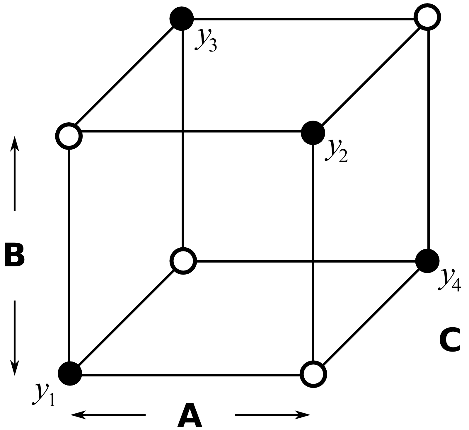
So this is our half-factorial designed experiment in 3 factors, but it only requires 4 experiments as shown by the open points in the figure. The experiments given by the solid points are not run.

What have we lost by running only half of the full factorial? Let’s write out the full design and matrix of all interactions, then construct the \(\mathbf{X}\) matrix for the least squares model.

Experiment	A	B	C	AB	AC	BC	ABC	Intercept
1	\(-\)	\(-\)	\(+\)	\(+\)	\(-\)	\(-\)	\(+\)	\(+\)
2	\(+\)	\(-\)	\(-\)	\(-\)	\(-\)	\(+\)	\(+\)	\(+\)
3	\(-\)	\(+\)	\(-\)	\(-\)	\(+\)	\(-\)	\(+\)	\(+\)
4	\(+\)	\(+\)	\(+\)	\(+\)	\(+\)	\(+\)	\(+\)	\(+\)

Before even constructing the \(\mathbf{X}\)-matrix, you can see that A=BC, and that B=AC and C=AB (this last association was intentional), and intercept I=ABC.

The least squares model would be:

\[\begin{split}\mathbf{y} &= \mathbf{X} \mathbf{b} + \mathbf{e}\\ y_i &= b_0 + b_A x_A + b_B x_B + b_C x_C + b_{AB} x_{AB} + b_{AC} x_{AC} + b_{BC} x_{BC} + b_{ABC} x_{ABC} + e_i\\ \begin{bmatrix} y_1\\ y_2\\ y_3 \\ y_4 \end{bmatrix} &= \begin{bmatrix} 1 & -1 & -1 & +1 & +1 & -1 & -1 & +1\\ 1 & +1 & -1 & -1 & -1 & -1 & +1 & +1\\ 1 & -1 & +1 & -1 & -1 & +1 & -1 & +1\\ 1 & +1 & +1 & +1 & +1 & +1 & +1 & +1 \end{bmatrix} \begin{bmatrix} b_0 \\ b_A \\ b_B \\ b_{C} \\ b_{AB} \\ b_{AC} \\ b_{BC} \\ b_{ABC} \end{bmatrix} + \begin{bmatrix} e_1\\ e_2\\ e_3 \\ e_4 \end{bmatrix}\end{split}\]

The \(\mathbf{X}\) matrix is not orthogonal anymore, because one or more columns are exactly identical to another column, also known as collinearity. Notice that 4 of the columns are the same as the other 4: we have perfect collinearity between 4 pairs of columns. Also note this system is underdetermined as there are more unknowns than equations.

For these reasons the least squares model cannot be solved by inverting the \(\mathbf{X}^T\mathbf{X}\) matrix. Prove it to yourself by using this code:

To resolve this problem we can reformulate the model to obtain independent columns, grouping together the columns which are identical. There are now 4 equations and 4 unknowns:

\[\begin{split}\mathbf{y} &= \mathbf{X} \mathbf{b} + \mathbf{e}\\ \begin{bmatrix} y_1\\ y_2\\ y_3 \\ y_4 \end{bmatrix} &= \begin{bmatrix} 1 & -1 & -1 & +1 \\ 1 & +1 & -1 & -1 \\ 1 & -1 & +1 & -1 \\ 1 & +1 & +1 & +1 \end{bmatrix} \begin{bmatrix} b_0 + b_{ABC} \\ b_A + b_{BC} \\ b_B + b_{AC} \\ b_{C} + b_{AB} \end{bmatrix} + \begin{bmatrix} e_1\\ e_2\\ e_3 \\ e_4 \end{bmatrix}\end{split}\]

Writing it this way clearly shows how the main effects and two-factor interactions are confounded.

\(b_0 + b_{ABC} = \widehat{\beta}_0 \rightarrow\) I + ABC

\(b_A + b_{BC} = \widehat{\beta}_A \rightarrow\) A + BC : this implies \(\beta_A\) estimates the A main effect and the BC interaction

\(b_B + b_{AC} = \widehat{\beta}_B \rightarrow\) B + AC

\(b_C + b_{AB} = \widehat{\beta}_C \rightarrow\) C + AB

It means we cannot separate, for example, the effect of the BC interaction from the main effect of A: the least-squares coefficient is a sum of both these effects. Similarly for the other pairs. This is why we say the factor A is confounded with the two-factor interaction BC. Factor B is confounded with AC, and factor C is confounded with AB. Also the intercept is not a pure estimate of the intercept; it is confounded with the 3-factor interaction ABC.

This is what we have lost by running a half-fraction: the benefit of doing fewer experiments is paid by the price of confounding within the factors we estimate.

We introduce the terminology that A is an alias for BC, similarly that B is an alias for AC, etc, because we cannot separate these aliased effects.