6.5.11. PCA example: analysis of spectral data
A data set, available on the dataset website, contains data on 460 tablets, measured at 650 different wavelengths.
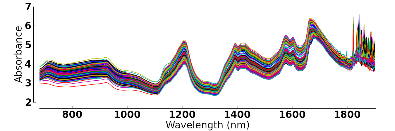
This R code will calculate principal components for this data:
# Read large data file
file <- 'http://openmv.net/file/tablet-spectra.csv'
spectra <- read.csv(file, header = FALSE, row.names = 1)
# Only extract 4 components, but
# center and scale the data before
# calculation the components
model.pca <- prcomp(spectra,
center = TRUE,
scale =TRUE,
rank. = 4)
summary(model.pca)
which gives this output:
Importance of first k=4 (out of 460) components:
PC1 PC2 PC3 PC4
Standard deviation 21.8835 10.9748 3.60075 3.27081
Proportion of Variance 0.7368 0.1853 0.01995 0.01646
Cumulative Proportion 0.7368 0.9221 0.94200 0.95846
The \(R^2_a\) (Cumulative Proportion
) values shows the first component explains 73.7% of the variability in \(\mathbf{X}\), the second explains an additional 18.5% for a cumulative total of 92.2%, and the third component explains an additional 1.99%. These three components together explain 94.2% of all the variation in \(\mathbf{X}\). This means we have reduced \(\mathbf{X}\) from a \(460 \times 650\) matrix to a \(460 \times 3\) matrix of scores, \(\mathbf{T}\), and a \(650 \times 3\) matrix of loadings, \(\mathbf{P}\). This is a large reduction in data size, with a minimal loss of information.
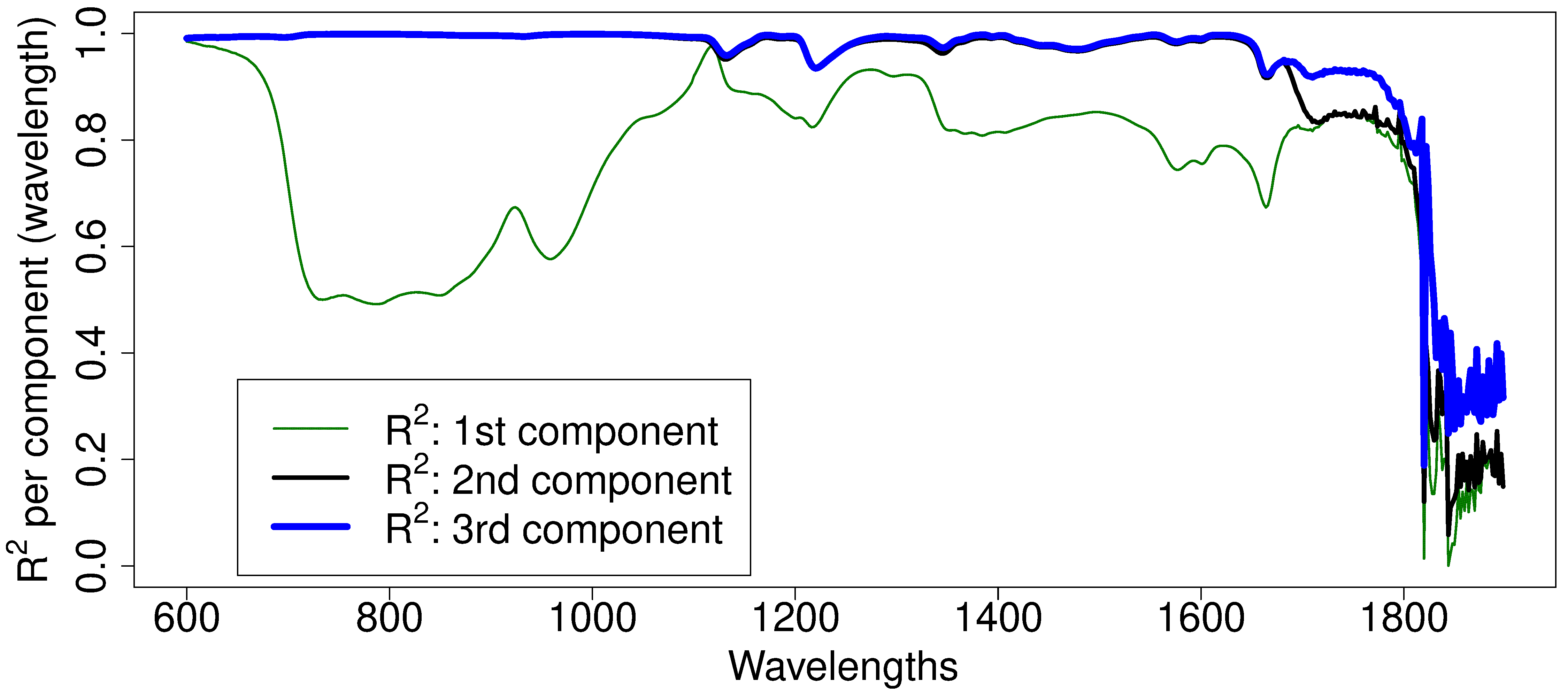
Let’s visually show what the \(R^2\) values are for each column. Shown below are these values for the first 3 components. The first component (green, thin line) explains certain regions of the spectra very well, particularly the region around 1100nm. Wavelengths beyond 1800 nm are not well explained at all. The second component is primarily responsible for explaining additional variability in the 700 to 1100nm region. The third component only seems to explain the additional variability from 1700 to 1800nm. Fitting a fourth component is only going to start fitting the noisy regions of the spectrum on the very right. For these data we could use 2 components for most applications, or perhaps 3 if the region between 1700 and 1800nm was also important.
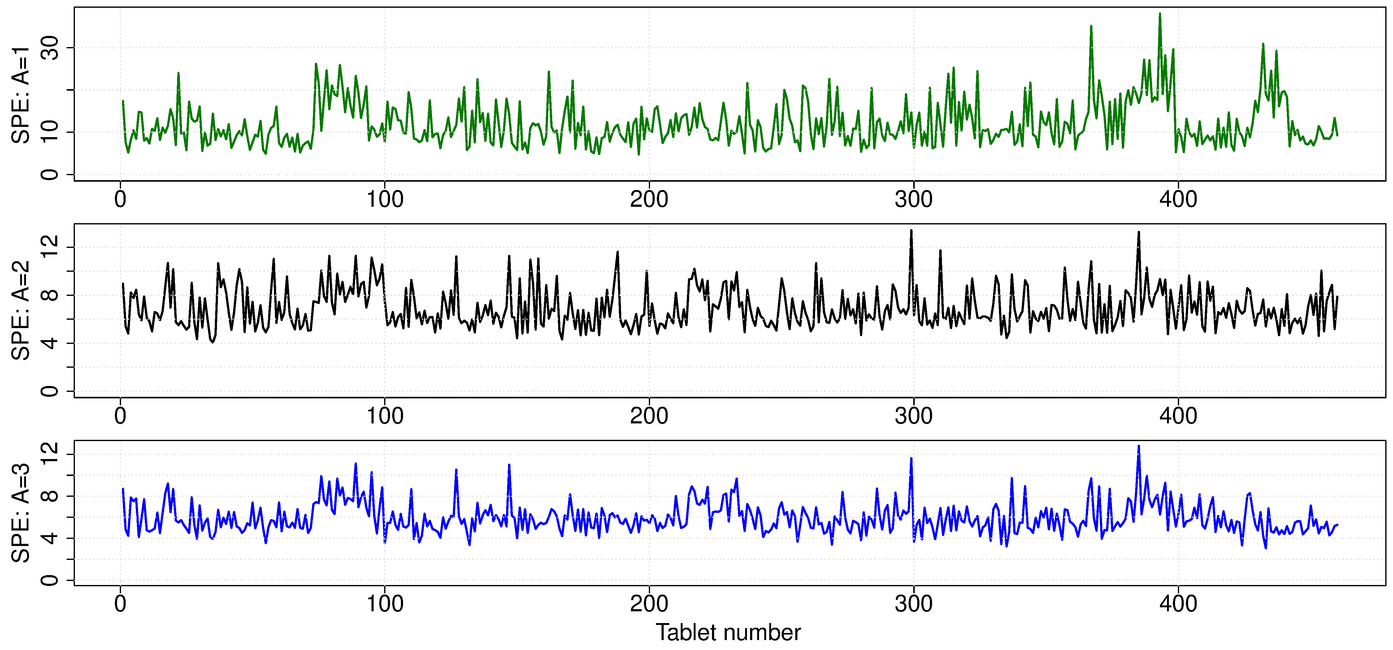
Finally, we can show the SPE plot for each observation. SPE values for each tablet become smaller and smaller as each successive component is added. Since each new component explains additional variance, the size of SPE must decrease. There don’t appear to be any major outliers off the model’s plane after the first component.
The code for the above plots is:
file <- 'http://openmv.net/file/tablet-spectra.csv'
spectra <- read.csv(file, header = FALSE, row.names = 1)
# Only extract 4 components, but
# center and scale the data before
# calculation the components
model.pca <- prcomp(spectra,
center = TRUE,
scale =TRUE,
rank. = 4)
spectra.P <- model.pca$rotation
spectra.T <- model.pca$x
# Baseline: mean and standard deviation per column
spectra.mean <- apply(spectra, 2, mean, na.rm=TRUE)
spectra.sd <- apply(spectra, 2, sd, na.rm=TRUE)
# Remove the calculated mean from each column (margin=2)
# by using the subtract function (FUN argument)
spectra.mc <- sweep(spectra, 2, spectra.mean, FUN='-')
# Scale each column, dividing by the standard deviation
spectra.mcuv <- sweep(spectra.mc, 2, spectra.sd, FUN='/')
# Baseline variance
spectra.X2 <- spectra.mcuv * spectra.mcuv
# A = 1
#------
a = 1
spectra.Xhat.a <- spectra.T[,seq(1,a)] %*% t(spectra.P[,seq(1,a)])
spectra.E <- spectra.mcuv - spectra.Xhat.a
spectra.E2 <- spectra.E * spectra.E
spectra.Xhat.a.2 <- spectra.Xhat.a * spectra.Xhat.a
SPE.1 <- sqrt(apply(spectra.E2, 1, sum))
R2.k.a <- apply(spectra.Xhat.a.2, 2, sum) / apply(spectra.X2, 2, sum)
wavelengths <- seq(600, 1898, 2)
plot(wavelengths, R2.k.a, col='darkgreen',
type='l', lwd=a*2, ylim=c(0,1),
ylab=expression("R"^2*" per component (wavelength)"),
xlab="Wavelengths")
# A = 2
#------
a = 2
spectra.Xhat.a <- spectra.T[,seq(1,a)] %*% t(spectra.P[,seq(1,a)])
spectra.E <- spectra.mcuv - spectra.Xhat.a
# mean for each row
spectra.E.mean <- apply(spectra.E, 1, mean, na.rm=TRUE)
spectra.E2 <- spectra.E * spectra.E
spectra.Xhat.a.2 <- spectra.Xhat.a * spectra.Xhat.a
SPE.2 <- sqrt(apply(spectra.E2, 1, sum))
R2.k.a <- apply(spectra.Xhat.a.2, 2, sum) / apply(spectra.X2, 2, sum)
lines(wavelengths, R2.k.a, col='black', type='l', lwd=a*2)
# A = 3
#------
a = 3
spectra.Xhat.a <- spectra.T[,seq(1,a)] %*% t(spectra.P[,seq(1,a)])
spectra.E <- spectra.mcuv - spectra.Xhat.a
spectra.E2 <- spectra.E * spectra.E
spectra.Xhat.a.2 <- spectra.Xhat.a * spectra.Xhat.a
SPE.3 <- sqrt(apply(spectra.E2, 1, sum))
R2.k.a <- apply(spectra.Xhat.a.2, 2, sum) / apply(spectra.X2, 2, sum)
lines(wavelengths, R2.k.a, col='blue', type='l', lwd=a*2)
legend(x=650, y=0.35,
legend=c(expression("R"^2*": 1st component"),
expression("R"^2*": 2nd component"),
expression("R"^2*": 3rd component")),
col=c("darkgreen", "black", "blue"),
lty=c(1, 1, 1), lwd=c(2,4,6), cex=1.0)
# SPE plot
N <- dim(spectra)[1]
layout(matrix(c(1,2,3), 3, 1))
plot(seq(1, N), SPE.1, col='darkgreen',
type='l', lwd=2, ylab="SPE: A=1",
ylim=c(0, max(SPE.1)))
plot(seq(1, N), SPE.2, col='black',
type='l', lwd=2, ylab="SPE: A=2",
ylim=c(0, max(SPE.2)))
plot(seq(1, N), SPE.2, col='blue',
type='l', lwd=2, ylab="SPE: A=3",
xlab="Tablet number", ylim=c(0, max(SPE.3)))