6.5.14. Algorithms to calculate (build) PCA models

The different algorithms used to build a PCA model provide a different insight into the model’s structure and how to interpret it. These algorithms are a reflection of how PCA has been used in different disciplines: PCA is called by different names in each area.

6.5.14.1. Eigenvalue decomposition

Note

The purpose of this section is not the theoretical details, but rather the interesting interpretation of the PCA model that we obtain from an eigenvalue decomposition.

Recall that the latent variable directions (the loading vectors) were oriented so that the variance of the scores in that direction were maximal. We can cast this as an optimization problem. For the first component:

\[\begin{split}\max \quad & \phi = \mathbf{t}'_1 \mathbf{t}_1 = \mathbf{p}'_1\mathbf{X}' \mathbf{X} \mathbf{p}_1 \\ \text{s.t.} \quad & \mathbf{p}'_1 \mathbf{p}_1 = 1\end{split}\]

This is equivalent to \(\max \,\, \phi = \mathbf{p}'_1 \mathbf{X}' \mathbf{X} \mathbf{p}_1 - \lambda \left(\mathbf{p}'_1 \mathbf{p}_1 - 1\right)\), because we can move the constraint into the objective function with a Lagrange multiplier, \(\lambda_1\).

The maximum value must occur when the partial derivatives with respect to \(\mathbf{p}_1\), our search variable, are zero:

\[\begin{split}\dfrac{\partial \phi}{\partial \mathbf{p}_1} &= \mathbf{0} = \mathbf{p}'_1 \mathbf{X}' \mathbf{X} \mathbf{p}_1 - \lambda_1\left(\mathbf{p}'_1 \mathbf{p}_1 - 1\right) \\ \mathbf{0} &= 2 \mathbf{X}' \mathbf{X} \mathbf{p}_1 - 2\lambda_1 \mathbf{p}_1 \\ \mathbf{0} &= (\mathbf{X}' \mathbf{X} - \lambda_1 I_{K\times K}) \mathbf{p}_1 \\ \mathbf{X}' \mathbf{X}\mathbf{p}_1 &= \lambda_1 \mathbf{p}_1\end{split}\]

which is just the eigenvalue equation, indicating that \(\mathbf{p}_1\) is the eigenvector of \(\mathbf{X}' \mathbf{X}\) and \(\lambda_1\) is the eigenvalue. One can show that \(\lambda_1 = \mathbf{t}'_1 \mathbf{t}_1\), which is proportional to the variance of the first component.

In a similar manner we can calculate the second eigenvalue, but this time we add the additional constraint that \(\mathbf{p}_1 \perp \mathbf{p}_2\). Writing out this objective function and taking partial derivatives leads to showing that \(\mathbf{X}' \mathbf{X}\mathbf{p}_2 = \lambda_2 \mathbf{p}_2\).

From this we learn that:

• The loadings are the eigenvectors of \(\mathbf{X}'\mathbf{X}\).

• Sorting the eigenvalues in order from largest to smallest gives the order of the corresponding eigenvectors, the loadings.

• We know from the theory of eigenvalues that if there are distinct eigenvalues, then their eigenvectors are linearly independent (orthogonal).

• We also know the eigenvalues of \(\mathbf{X}'\mathbf{X}\) must be real values and positive; this matches with the interpretation that the eigenvalues are proportional to the variance of each score vector.

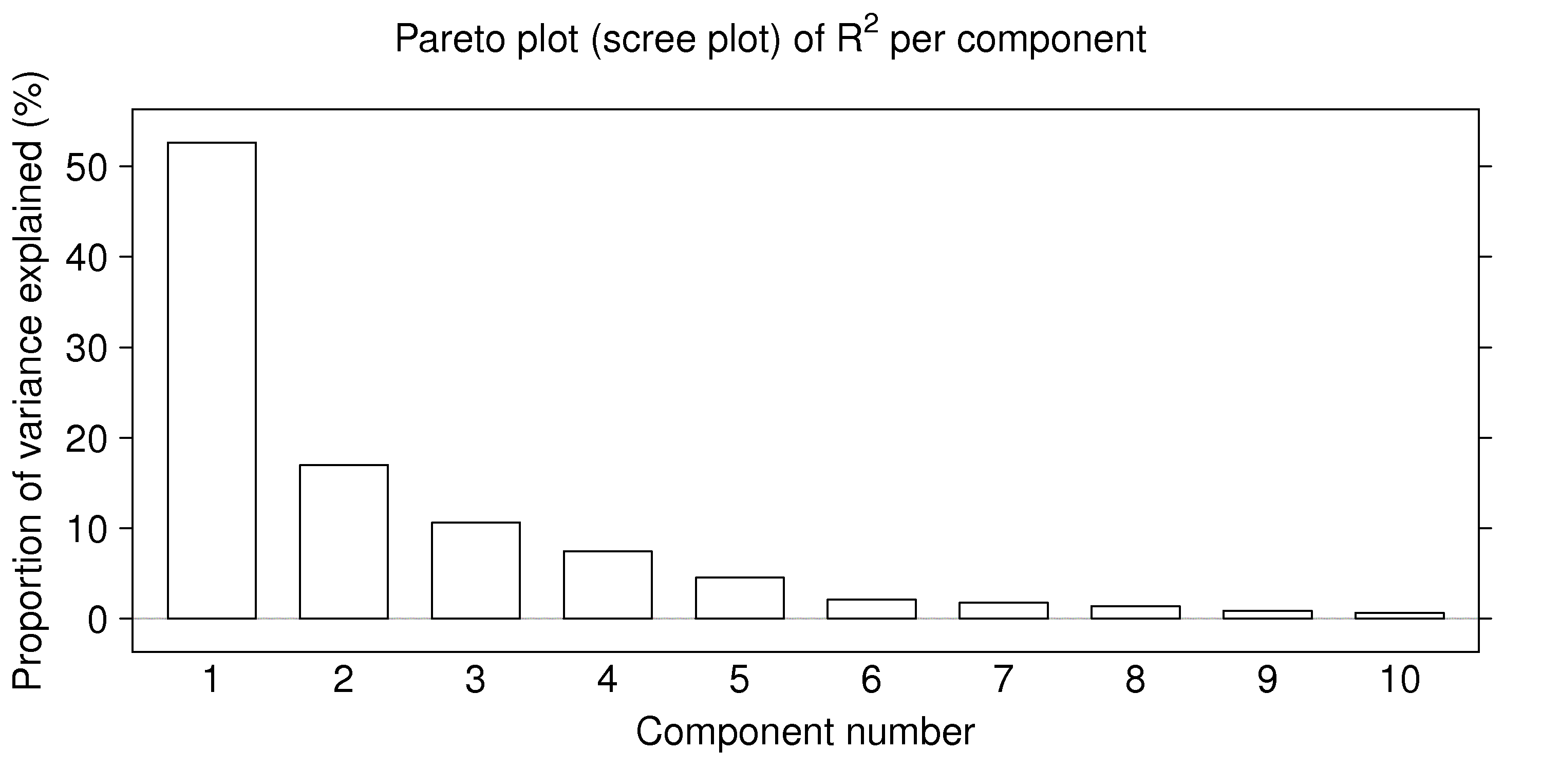
• Also, the sum of the eigenvalues must add up to sum of the diagonal entries of \(\mathbf{X}'\mathbf{X}\), which represents of the total variance of the \(\mathbf{X}\) matrix, if all eigenvectors are extracted. So plotting the eigenvalues is equivalent to showing the proportion of variance explained in \(\mathbf{X}\) by each component. This is not necessarily a good way to judge the number of components to use, but it is a rough guide: use a Pareto plot of the eigenvalues (though in the context of eigenvalue problems, this plot is called a scree plot).

  

The general approach to using the eigenvalue decomposition would be:

1. Preprocess the raw data, particularly centering and scaling, to create a matrix \(\mathbf{X}\).

2. Calculate the correlation matrix \(\mathbf{X}'\mathbf{X}\).

3. Calculate the eigenvectors and eigenvalues of this square matrix and sort the results from largest to smallest eigenvalue.

4. A rough guide is to retain only the first \(A\) eigenvectors (loadings), using a Scree plot of the eigenvalues as a guide. Alternative methods to determine the number of components are described in the section on cross-validation and randomization.

However, we should note that calculating the latent variable model using an eigenvalue algorithm is usually not recommended, since it calculates all eigenvectors (loadings), even though only the first few will be used. The maximum number of components possible is \(A_\text{max} = \min(N, K)\). Also, the default eigenvalue algorithms in software packages cannot handle missing data.

6.5.14.2. Singular value decomposition

The singular value decomposition (SVD), in general, decomposes a given matrix \(\mathbf{X}\) into three other matrices:

\[\mathbf{X} = \mathbf{U} \mathbf{\Sigma} \mathbf{V}'\]

Matrices \(\mathbf{U}\) and \(\mathbf{V}\) are orthonormal (each column has unit length and each column is orthogonal to the others), while \(\mathbf{\Sigma}\) is a diagonal matrix. The relationship to principal component analysis is that:

\[\mathbf{X} = \mathbf{T} \mathbf{P}'\]

where matrix \(\mathbf{P}\) is also orthonormal. So taking the SVD on our preprocessed matrix \(\mathbf{X}\) allows us to get the PCA model by setting \(\mathbf{P} = \mathbf{V}\), and \(\mathbf{T} = \mathbf{U} \mathbf{\Sigma}\). The diagonal terms in \(\mathbf{\Sigma}\) are related to the variances of each principal component and can be plotted as a scree plot, as was done for the eigenvalue decomposition.

Like the eigenvalue method, the SVD method calculates all principal components possible, \(A=\min(N, K)\), and also cannot handle missing data by default.

6.5.14.3. Non-linear iterative partial least-squares (NIPALS)

The non-linear iterative partial least squares (NIPALS) algorithm is a sequential method of computing the principal components. The calculation may be terminated early, when the user deems that enough components have been computed. Most computer packages tend to use the NIPALS algorithm as it has two main advantages: it handles missing data and calculates the components sequentially.

The purpose of considering this algorithm here is three-fold: it gives additional insight into what the loadings and scores mean; it shows how each component is independent of (orthogonal to) the other components, and it shows how the algorithm can handle missing data.

The algorithm extracts each component sequentially, starting with the first component, direction of greatest variance, and then the second component, and so on.

We will show the algorithm here for the \(a^\text{th}\) component, where \(a=1\) for the first component. The matrix \(\mathbf{X}\) that we deal with below is the preprocessed, usually centered and scaled matrix, not the raw data.

1. The NIPALS algorithm starts by arbitrarily creating an initial column for \(\mathbf{t}_a\). You can use a column of random numbers, or some people use a column from the \(\mathbf{X}\) matrix; anything can be used as long as it is not a column of zeros.

2. Then we take every column in \(\mathbf{X}\), call it \(\mathbf{X}_k\), and regress it onto this initial column \(\mathbf{t}_a\); store the regression coefficient as the entry in \(p_{k,a}\). What this means, and it is illustrated below, is that we perform an ordinary least squares regression (\(\mathbf{y} = \beta \mathbf{x}\)), except our \(\mathrm{x}\)-variable is this column of \(\mathbf{t}_a\) values, and our \(\mathrm{y}\)-variable is the particular column from \(\mathbf{X}\).

   

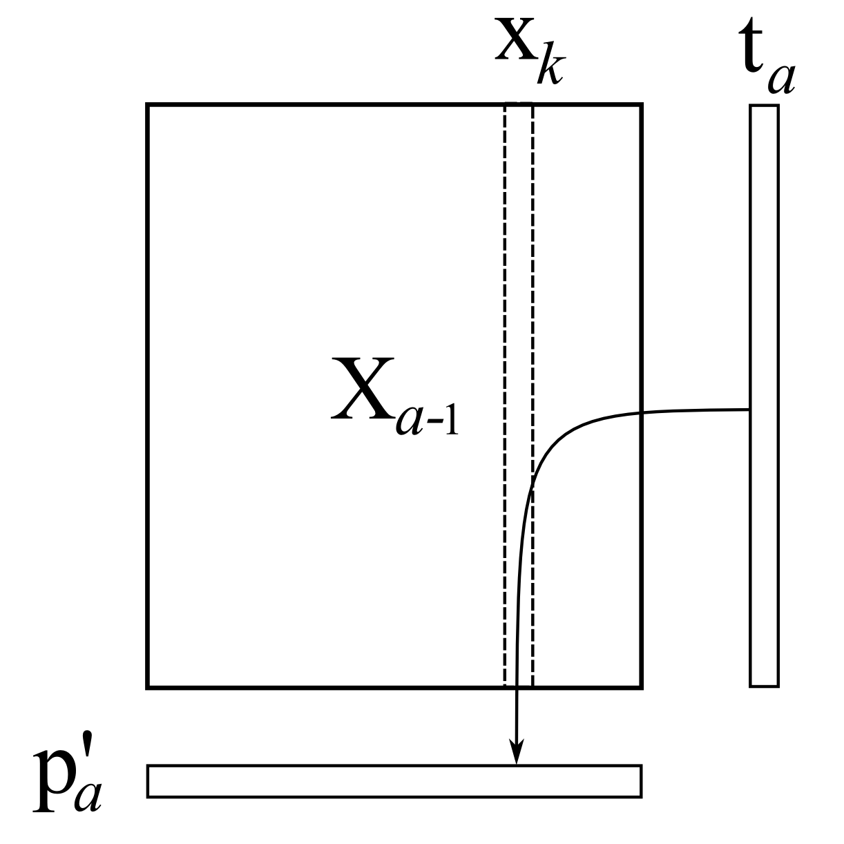
   For ordinary least squares, you will remember that the solution for this regression problem is \(\widehat{\beta} = \dfrac{\mathbf{x'y}}{\mathbf{x'x}}\). Using our notation, this means:

   \[p_{k,a} = \dfrac{\mathbf{t}'_a \mathbf{X}_k}{\mathbf{t}'_a\mathbf{t}_a}\]

   This is repeated for each column in \(\mathbf{X}\) until we fill the entire vector \(\mathbf{p}_k\). This is shown in the illustration where each column from \(\mathbf{X}\) is regressed, one at a time, on \(\mathbf{t}_a\), to calculate the loading entry, \(p_{k,a}\) In practice we don’t do this one column at time; we can regress all columns in \(\mathbf{X}\) in go: \(\mathbf{p}'_a = \dfrac{1}{\mathbf{t}'_a\mathbf{t}_a} \cdot \mathbf{t}'_a \mathbf{X}_a\), where \(\mathbf{t}_a\) is an \(N \times 1\) column vector, and \(\mathbf{X}_a\) is an \(N \times K\) matrix, explained more clearly in step 6.

3. The loading vector \(\mathbf{p}'_a\) won’t have unit length (magnitude) yet. So we simply rescale it to have magnitude of 1.0:

   \[\mathbf{p}'_a = \dfrac{1}{\sqrt{\mathbf{p}'_a \mathbf{p}_a}} \cdot \mathbf{p}'_a\]

4. The next step is to regress every row in \(\mathbf{X}\) onto this normalized loadings vector. As illustrated below, in our linear regression the rows in \(\mathbf{X}\) are our \(\mathrm{y}\)-variable each time, while the loadings vector is our \(\mathrm{x}\)-variable. The regression coefficient becomes the score value for that \(i^\text{th}\) row:

   
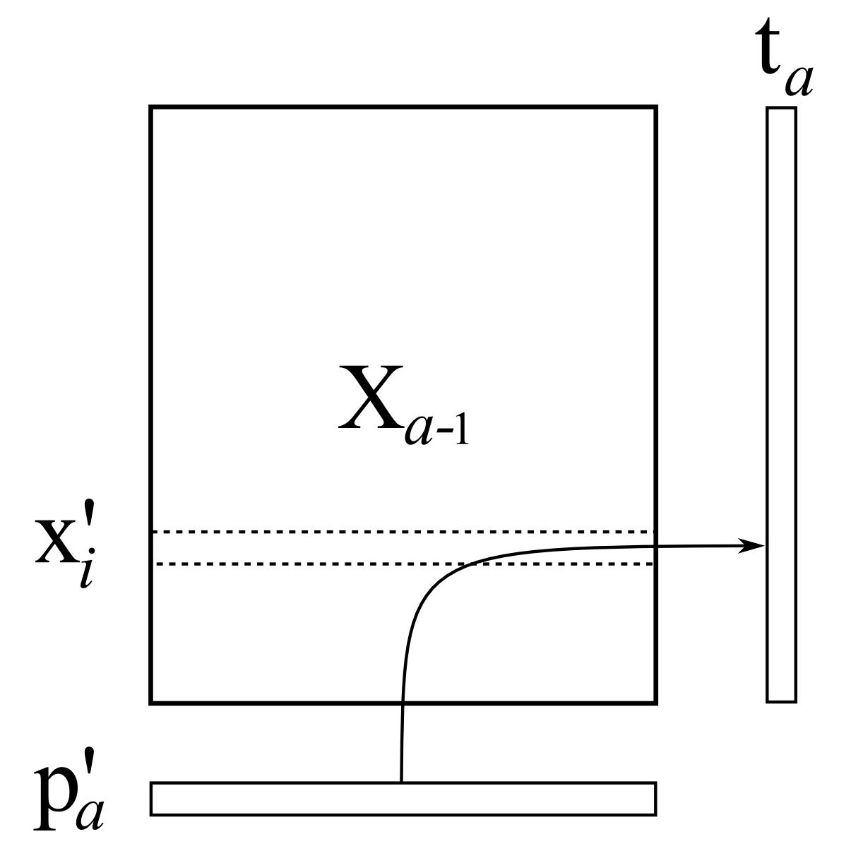   \[t_{i,a} = \dfrac{\mathbf{x}'_i \mathbf{p}_a}{\mathbf{p}'_a\mathbf{p}_a}\]

   where \(\mathbf{x}'_i\) is an \(K \times 1\) column vector. We can combine these \(N\) separate least-squares models and calculate them in one go to get the entire vector, \(\mathbf{t}_a = \dfrac{1}{\mathbf{p}'_a\mathbf{p}_a} \cdot \mathbf{X} \mathbf{p}_a\), where \(\mathbf{p}_a\) is a \(K \times 1\) column vector.

5. We keep iterating steps 2, 3 and 4 until the change in vector \(\mathbf{t}_a\) from one iteration to the next is small (usually around \(1 \times 10^{-6}\) to \(1 \times 10^{-9}\)). Most data sets require no more than 200 iterations before achieving convergence.

6. On convergence, the score vector and the loading vectors, \(\mathbf{t}_a\) and \(\mathbf{p}_a\) are stored as the \(a^\text{th}\) column in matrix \(\mathbf{T}\) and \(\mathbf{P}\) respectively. We then deflate the \(\mathbf{X}\) matrix. This crucial step removes the variability captured in this component (\(\mathbf{t}_a\) and \(\mathbf{p}_a\)) from \(\mathbf{X}\):

   \[\begin{split}\mathbf{E}_a &= \mathbf{X}_{a} - \mathbf{t}_a \mathbf{p}'_a \\ \mathbf{X}_{a+1} &= \mathbf{E}_a\end{split}\]

   For the first component, \(\mathbf{X}_{a}\) is just the preprocessed raw data. So we can see that the second component is actually calculated on the residuals \(\mathbf{E}_1\), obtained after extracting the first component.

   This is called deflation, and nicely shows why each component is orthogonal to the others. Each subsequent component is only seeing variation remaining after removing all the others; there is no possibility that two components can explain the same type of variability.

   After deflation we go back to step 1 and repeat the entire process for the next component. Just before accepting the new component we can use a test, such as a randomization test, or cross-validation, to decide whether to keep that component or not.

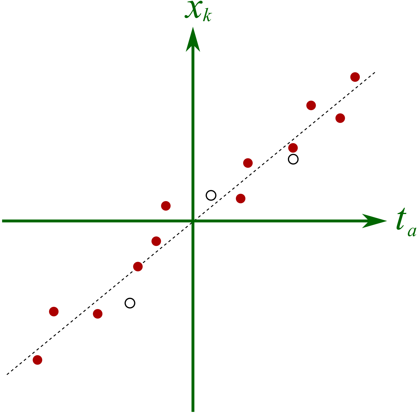
The final reason for outlining the NIPALS algorithm is to show one way in which missing data can be handled. All that step 2 and step 4 are doing is a series of regressions. Let’s take step 2 to illustrate, but the same idea holds for step 4. In step 2, we were regressing columns from \(\mathbf{X}\) onto the score \(\mathbf{t}_a\). We can visualize this for a hypothetical system below

There are 3 missing observations (open circles), but despite this, the regression’s slope can still be adequately determined. The slope is unlikely to change by very much if we did have the missing values. In practice though we have no idea where these open circles would fall, but the principle is the same: we calculate the slope coefficient just ignoring any missing entries.

In summary:

• The NIPALS algorithm computes one component at a time. The first component computed is equivalent to the \(\mathbf{t}_1\) and \(\mathbf{p}_1\) vectors that would have been found from an eigenvalue or singular value decomposition.

• The algorithm can handle missing data in \(\mathbf{X}\).

• The algorithm always converges, but the convergence can sometimes be slow.

• It is also known as the Power algorithm to calculate eigenvectors and eigenvalues.

• It works well for very large data sets.

• It is used by most software packages, especially those that handle missing data.

• Of interest: it is well known that Google used this algorithm for the early versions of their search engine, called PageRank.