
 Download PDF of entire book
5.24. Exercises
Question
These readings are to illustrate the profound effect that designed experiments have had in some areas.
Application of Statistical Design of Experiments Methods in Drug Discovery and using DOE for high-throughput screening to locate new drug compounds.
High traffic websites offer a unique opportunity to perform testing and optimization. This is because each visitor to the site is independent of the others (randomized), and these tests can be run in parallel. Read more in this brief writeup on how Google uses testing tools to optimize YouTube, one of their web properties. Unfortunately they use the term “multivariate” incorrectly - a better term is “multi-variable”; nevertheless, the number of factors and combinations to be tested is large. It’s well known that fractional factorial methods are used to analyze these data.
See three chemical engineering examples of factorial designs in Box, Hunter, and Hunter: Chapter 11 (1st edition), or page 173 to 183 in the second edition.
Question
Your family runs a small business selling low dollar value products over the web. They want to improve sales. There is a known effect from the day of the week, so to avoid that effect they run the following designed experiment every Tuesday for the past eight weeks. The first factor of interest is whether to provide free shipping over $30 or over $50. The second factor is whether or not the purchaser must first create a profile (user name, password, address, etc) before completing the transaction. The purchaser can still complete their transaction without creating a profile.
These are the data collected:
Date
Free shipping over …
Profile required before transaction
Total sales made
05 January 2010
$30
Yes
$ 3275
12 January 2010
$50
No
$ 3594
19 January 2010
$50
No
$ 3626
26 January 2010
$30
No
$ 3438
02 February 2010
$50
Yes
$ 2439
09 February 2010
$30
No
$ 3562
16 February 2010
$30
Yes
$ 2965
23 February 2010
$50
Yes
$ 2571
You can check your analysis with Factorial, the designed-experiments app, which opens these eight days with their sales.
Calculate the average response from replicate experiments to calculate the 4 corner points.
Calculate and interpret the main effects in the design.
Show the interaction plot for the 2 factors.
We will show in the next class how to calculate confidence intervals for each effect, but would you say there is an interaction effect here? How would you interpret the interaction (whether there is one or not)?
What is the recommendation to increase sales?
Calculate the main effects and interactions by hand using a least squares model. You may confirm your result using software, but your answer should not just be the computer software output.
Solution
This is a \(2^2\) factorial system with a replicate at each point. Average the replicate points and then calculate the main effects and other terms for this system. You will get the same result if you analyze it as two separate factorials and then average the results - it’s just more work that way though.
The experiment results in standard form with 4 corner points:
A
B
Average sales
\(-\)
\(-\)
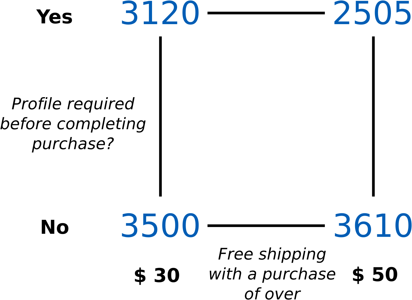
\(\tfrac{1}{2}\left(3438+3562\right) = \$ 3,500\)
\(+\)
\(-\)
\(\tfrac{1}{2}\left(3594+3626\right) = \$ 3,610\)
\(-\)
\(+\)
\(\tfrac{1}{2}\left(3275+2965\right) = \$ 3,120\)
\(+\)
\(+\)
\(\tfrac{1}{2}\left(2439+2571\right) = \$ 2,505\)
where \(\mathbf{A}\) = free shipping over $30 (low level) and $50 (high level), and let \(\mathbf{B} = -1\) if no profile is required, or \(+1\) if a profile is required before completing the transaction.
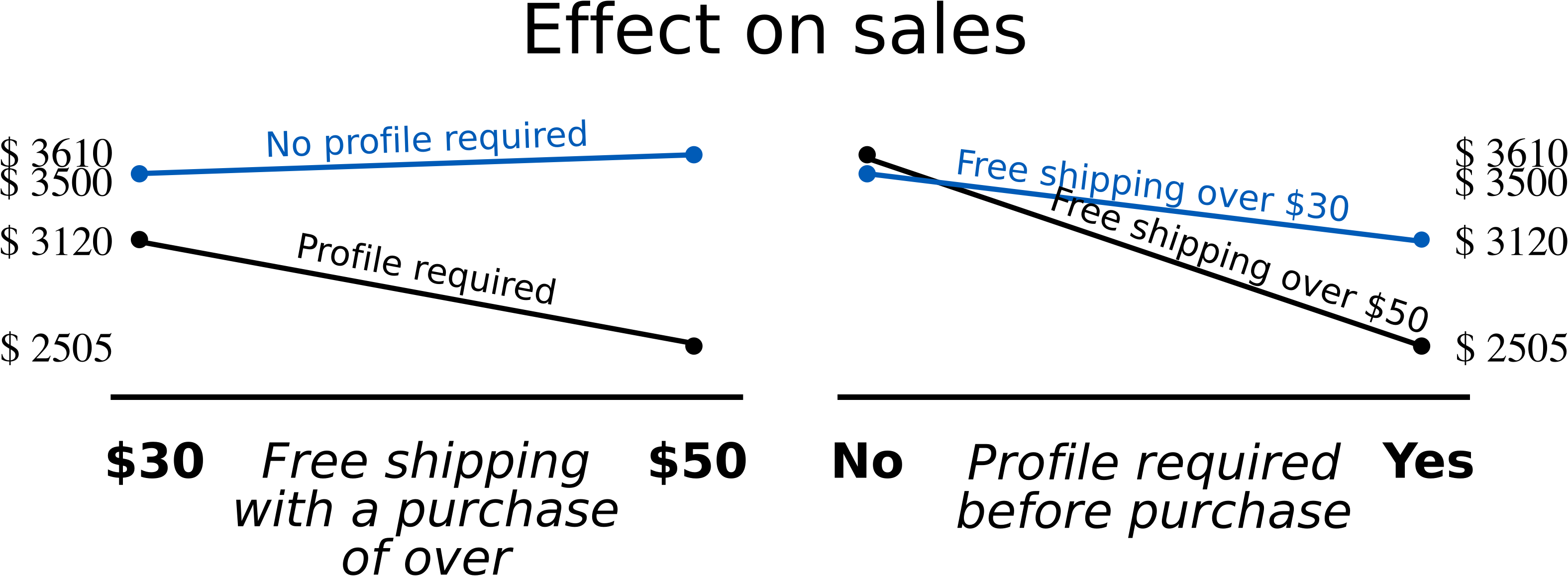
The main effect for free shipping (A) is = \(\tfrac{1}{2}(3610 - 3500 + 2505 - 3120) = \dfrac{-505}{2} = -252.50\)
This indicates that sales decrease by $252.50, on average, when going from free shipping over $30 to $50. One might expect, within reason, that higher sales are made when the free shipping value is higher (people add purchases so they reach the free shipping limit). That is shown by the small increase in sales, $110, from raising the threshold to $50 when no profile is required. However when a profile is required, we see the opposite: a drop in sales!
The main effect of creating a profile \(\mathbf{B} = \tfrac{1}{2}(3120 - 3500 + 2505 - 3610) = \dfrac{-1485}{2} = -742.50\)
Indicating that sales drop by $742.50 on average when requiring a profile before completing the transaction vs not requiring a profile. The drop in sales is less when offering free shipping over $30 than when free shipping is for $50 or more in purchases.
Not required for this question, but one of the best ways to visualize a small factorial, or a subset of a larger factorial, is with a cube plot:
The interaction plot which visually shows the main effects described above is:
The interaction term can be calculated in two ways, both giving the same answer. Only one way is shown here:
A at high B: -$615.00
A at low B: $ 110.00
AB interaction = \(\tfrac{1}{2}\left(-615 - 110\right) = \dfrac{-725}{2} = - 362.50\)
This interaction term is larger than one of the main effects, so I would judge this to be important. Also, it is roughly 10% of the \(y_i =\) daily sales values, so it is definitely important.
In part 2 we showed the main effect of requiring a profile is to decrease sales. The strong negative interaction term here indicates that sales are even further reduced when free shipping is over $50, rather than $30. Maybe it’s because customers “give up” making their purchase when free shipping is at a higher amount and they need to create a profile - perhaps they figure this isn’t worth it. If they get free shipping over $30, the penalty of creating a profile is not as great anymore. This last effect might be considered counterintuitive - but I’m not an expert on why people buy stuff.
In general, an interaction term indicates that the usual main effects are increased or decreased more or less than they would have been when acting on their own.
Sales can be definitely increased by not requiring the user to create a profile before completing the transaction (creating a profile is a strong deterrent to increasing sales, whether free shipping over $30 or $50 is offered). The effect of free shipping when not requiring a profile is small. The raw data for the case when no profile was required (below), show slightly higher sales when free shipping over $50 is required. Further experimentation to assess if this is significant or not would be required.
Date
Free shipping over …
Profile required before transaction
Total sales made that day
12 January 2010
$50
No
$ 3594
19 January 2010
$50
No
$ 3626
26 January 2010
$30
No
$ 3438
09 February 2010
$30
No
$ 3562
A least squares model can be calculated from the average of each replicate. Then there are 4 observations and 4 unknowns. Using the design matrix, in standard order, we can set up the following least squares model:
\[\begin{split}\mathbf{y} &= \mathbf{X}\mathbf{b} + \mathbf{e} \\ \begin{bmatrix} y_1 \\ y_2 \\ y_3 \\ y_4 \end{bmatrix} &= \begin{bmatrix} 1 & -1 & -1 & +1 \\ 1 & +1 & -1 & -1 \\ 1 & -1 & +1 & -1 \\ 1 & +1 & +1 & +1 \end{bmatrix} \begin{bmatrix} b_0 \\ b_\mathbf{A} \\ b_\mathbf{B} \\ b_\mathbf{AB} \end{bmatrix} + \begin{bmatrix} e_1 \\ e_2 \\ e_3 \\ e_4 \end{bmatrix} \\ \begin{bmatrix} 3500 \\ 3610 \\ 3120 \\ 2505 \end{bmatrix} &= \begin{bmatrix} 1 & -1 & -1 & +1 \\ 1 & +1 & -1 & -1 \\ 1 & -1 & +1 & -1 \\ 1 & +1 & +1 & +1 \end{bmatrix} \begin{bmatrix} b_0 \\ b_\mathbf{A} \\ b_\mathbf{B} \\ b_\mathbf{AB} \end{bmatrix} + \begin{bmatrix} e_1 \\ e_2 \\ e_3 \\ e_4 \end{bmatrix}\end{split}\]And solving the regression coefficients (note the orthogonality in the \(\mathbf{X}^T\mathbf{X}\) matrix):
\[\begin{split}\mathbf{b} &= \left(\mathbf{X}^T\mathbf{X}\right)^{-1}\mathbf{X}^T\mathbf{y}\\ \mathbf{b} &= \left(\begin{matrix} 4 & 0 & 0 & 0 \\ 0 & 4 & 0 & 0 \\ 0 & 0 & 4 & 0 \\ 0 & 0 & 0 & 4 \end{matrix}\right)^{-1} \begin{bmatrix} + 3500 + 3610 + 3120 + 2505 \\ -3500 + 3610 - 3120 + 2505 \\ -3500 - 3610 + 3120 + 2505 \\ + 3500 - 3610 - 3120 + 2505 \end{bmatrix} \\ \mathbf{b} &= \begin{bmatrix} \tfrac{1}{4} & 0 & 0 & 0 \\ 0 & \tfrac{1}{4} & 0 & 0 \\ 0 & 0 &\tfrac{1}{4} & 0 \\ 0 & 0 & 0 & \tfrac{1}{4} \end{bmatrix} \begin{bmatrix} 12735 \\ -505 \\ -1485 \\ -725 \end{bmatrix} \\ \begin{bmatrix} b_0 \\ b_\mathbf{A} \\ b_\mathbf{B} \\ b_\mathbf{AB} \end{bmatrix} &= \begin{bmatrix} 3184 \\ -126 \\ -371 \\ -181 \end{bmatrix}\end{split}\]The final model is \(y = 3184 - 126 x_\mathrm{A} - 371 x_\mathrm{B} - 181 x_\mathrm{AB}\).
Compare the values in the \(\mathbf{X}^T\mathbf{y}\) vector to the calculations for the main effects and interactions to see the similarity. The least squares model parameters are half the size of the main effects and interactions reported above, because of how the parameters are interpreted in the least squares model.
Particularly the effect of requiring a profile, \(x_B\), is to reduce sales by \(2 \times $371 = $ 742\).
Question
More readings:
It is worth reading this paper by Bisgaard to see how the same tools shown in these notes were used to solve a real industrial problem: designed experiments, autocorrelation plots, data visualization, and quality control charts. Also he describes how the very real pressure from managers, time-constraints and interactions with team-members impacted the work.
“The Quality Detective: A Case Study” (and discussion), Philosophical Transactions of the Royal Society A, 327, 499-511, 1989.
George Box, The R. A. Fisher Memorial Lecture, 1988, “Quality Improvement - An Expanding Domain for the Application of Scientific Method”, Philosophical Transactions of the Royal Society - A, 327: pages 617-630, 1989.
Question
Note
This is a tutorial-type question: all the sub-questions build on each other. All questions deal with a hypothetical bioreactor system, and we are investigating four factors:
A = feed rate: slow or medium
B = initial inoculant size (300g or 700g)
C = feed substrate concentration (40 g/L or 60 g/L)
D = dissolved oxygen set-point (4mg/L or 6 mg/L)
The 16 experiments from a full factorial, \(2^4\), were randomly run, and the yields from the bioreactor, \(y\), are reported here in standard order: y = [60, 59, 63, 61, 69, 61, 94, 93, 56, 63, 70, 65, 44, 45, 78, 77].
You can check your analysis with Factorial, the designed-experiments app, which opens these 16 runs with their yields.
Calculate the 15 main effects and interactions and the intercept, using computer software.
Use a Pareto-plot to identify the significant effects. What would be your advice to your colleagues to improve the yield?
Refit the model using only the significant terms identified in the second question.
Explain why you don’t actually have to recalculate the least squares model parameters.
Compute the standard error and confirm that the effects are indeed significant at the 95% level.
Write down the exact settings for A, B, C, and D you would provide to the graduate student running a half-fraction in 8 runs for this system.
Before the half-fraction experiments are even run you can calculate which variables will be confounded (aliased) with each other. Report the confounding pattern for these main effects and for these two-factor interactions. Your answer should be in this format:
Generator =
Defining relationship =
Confounding pattern:
\(\widehat{\beta}_\mathbf{A} \rightarrow\)
\(\widehat{\beta}_\mathbf{B} \rightarrow\)
\(\widehat{\beta}_\mathbf{C} \rightarrow\)
\(\widehat{\beta}_\mathbf{D} \rightarrow\)
\(\widehat{\beta}_\mathbf{AB} \rightarrow\)
\(\widehat{\beta}_\mathbf{AC} \rightarrow\)
\(\widehat{\beta}_\mathbf{AD} \rightarrow\)
\(\widehat{\beta}_\mathbf{BC} \rightarrow\)
\(\widehat{\beta}_\mathbf{BD} \rightarrow\)
\(\widehat{\beta}_\mathbf{CD} \rightarrow\)
Now use the 8 yield values corresponding to your half fraction, and calculate as many parameters (intercept, main effects, interactions) as you can.
Report their numeric values.
Compare your parameters from this half-fraction (8 runs) to those from the full factorial (16 runs). Was much lost by running the half fraction?
What was the resolution of the half-fraction?
What is the projectivity of this half-fraction? And what does this mean in light of the fact that factor A was shown to be unimportant?
Suppose you need an estimate of factor C that is not aliased with ABD. Obviously in this problem, the foldover set of experiments to run would be the other half-fraction. Use the foldover method for de-aliasing a single main effect to show that the other 8 experiments to de-alias factor C would just be the other 8 experiments not included in your first half-fraction.
Solution
Using the computer code (at the end of the question), we found the complete model for all effects and interaction as:
\[\begin{split}\hat{y} &= 66.125 - 0.625 x_A + 9 x_B + 4 x_C - 3.875 x_D - 0.5 x_Ax_B - 0.5 x_Ax_C + 0.875 x_Ax_D + 6.375 x_Bx_C + 1.25 x_Bx_D - 5.25 x_Cx_D\\ &+ 1.125 x_Ax_Bx_C - 1.25 x_Ax_Bx_D + 0.25 x_Ax_Cx_D - 0.125 x_Bx_Cx_D + 0.125 x_Ax_Bx_Cx_D\end{split}\]The Pareto plot shows the important main effects are B, C, D and these two-factor interactions: BC and CD.
The advice to improve yield would be to:
A: use either the slow or medium feedrate, whichever has the better process economics
B: operate with the larger inoculant size: 700g
C: use a higher feed concentration 60 g/L
D: use the lower dissolved oxygen set point of 4 mg/L
BC: in this case the BC interaction works in our favour (high \(\times\) high)
CD: the CD interaction also works in our favour, since -5.25 \(\times\) (+1) \(\times\) (-1) leads to an increased yield.
At these conditions the expected yield is in the region of 93 to 94% (runs 7 and 8 from the standard order).

The model does not have to be refitted because the columns in matrix \(\mathbf{X}\) are orthogonal, meaning that the coefficient estimates do not depend on the levels of any other variables.
By dropping out the insignificant coefficients and keeping only the 5 parameters from the Pareto plus the intercept, we have 6 parameters, 16 data points, so 10 degrees of freedom. The residual vector is found from \(\mathbf{e} = \mathbf{y} - \hat{\mathbf{y}}\), where \(\hat{\mathbf{y}} = \underbrace{\mathbf{X}_{\text{sub}}}_{16 \times 6} \underbrace{\mathbf{b}_\text{sub}}_{6 \times 1}\).
The subset matrix of \(\mathbf{X}_{\text{sub}}\) is found by sub-sampling from the full \(16 \times 16\) matrix; similarly for the coefficient vector \(\mathbf{b}\). From this we can calculate:
The standard error is \(S_E = 3.1\), which is pretty tight, considering the ranges of y-values in the data set
The critical \(t\)-value for the 95% confidence level = 2.23
The variances of the parameters in the model are the diagonal of \(\left(\mathbf{X}^T\mathbf{X}\right)^{-1}S_E^2\), and \(\mathbf{X}^T\mathbf{X} = 16\mathbf{I}\) because the columns are orthogonal. So \(S_E(b_i) = \sqrt{\dfrac{3.1^2}{16}}\) = 0.78.
The confidence intervals for each of the significant effects are:
\[\begin{split}\begin{array}{rcl} 7.3 \leq &\beta_B &\leq 10.7 \\ 2.3 \leq &\beta_C &\leq 5.7\\ -5.6 \leq &\beta_D &\leq -2.1\\ 4.6 \leq &\beta_{BC} &\leq 8.1\\ -7.0 \leq &\beta_{CD} &\leq -3.5 \end{array}\end{split}\]
A half-fraction of a \(2^4\) factorial has 8 experiments. We can generate the levels for 3 of the factors, A, B and C from a full factorial in these 8 runs. The generating term for the fourth factor D is best set to the highest-order interaction, the ABC term.
Using that concept, we would ask the graduate student to run these 8 experiments in random order:
Experiment
Feed rate
Inoculant size
Feed concentration
DO set point
1
Slow
300g
40 g/L
4 mg/L
2
Medium
300g
40 g/L
6 mg/L
3
Slow
700g
40 g/L
6 mg/L
4
Medium
700g
40 g/L
4 mg/L
5
Slow
300g
60 g/L
6 mg/L
6
Medium
300g
60 g/L
4 mg/L
7
Slow
700g
60 g/L
4 mg/L
8
Medium
700g
60 g/L
6 mg/L
Factorial, the designed-experiments app, opens these eight runs with their yields.
Generator = D = ABC
Defining relationship = I = ABCD
Confounding pattern:
\(\widehat{\beta}_\mathbf{A} \rightarrow\) A + BCD
\(\widehat{\beta}_\mathbf{B} \rightarrow\) B + ACD
\(\widehat{\beta}_\mathbf{C} \rightarrow\) C + ABD
\(\widehat{\beta}_\mathbf{D} \rightarrow\) D + ABC
\(\widehat{\beta}_\mathbf{AB} \rightarrow\) AB + CD
\(\widehat{\beta}_\mathbf{AC} \rightarrow\) AC + BD
\(\widehat{\beta}_\mathbf{AD} \rightarrow\) AD + BC
\(\widehat{\beta}_\mathbf{BC} \rightarrow\) BC + AD
\(\widehat{\beta}_\mathbf{BD} \rightarrow\) BD + AC
\(\widehat{\beta}_\mathbf{CD} \rightarrow\) CD + AB
Selecting the rows from the full factorial design which correspond to the 8 runs from the half factorial we get \(y = [60, 63, 70, 61, 44, 61, 94, 77]\) corresponding to the table order in part 4.
Then forming the \(\mathbf{X}\) matrix from the table in part 4 we solve for the parameters as follows:
\(\widehat{b}_0 = 66.25 \rightarrow\) I + ABCD
\(\widehat{b}_\mathbf{A} = -0.75 \rightarrow\) A + BCD (previous estimate for A was -0.625)
\(\widehat{b}_\mathbf{B} = 9.25 \rightarrow\) B + ACD (previous estimate for B was 9.0)
\(\widehat{b}_\mathbf{C} = 2.75 \rightarrow\) C + ABD (previous estimate for C was 4.0)
\(\widehat{b}_\mathbf{D} = -2.75 \rightarrow\) D + ABC (previous estimate for D was -3.875)
\(\widehat{b}_\mathbf{AB} = -5.75 \rightarrow\) AB + CD (previous estimate for AB was insignificant, while CD was -5.25)
\(\widehat{b}_\mathbf{AC} = 0.75 \rightarrow\) AC + BD (previous estimates for both AC and BD were insignificant)
\(\widehat{b}_\mathbf{AD} = 7.25 \rightarrow\) AD + BC (previous estimate for AD was insignificant, while BC was 6.375)
You can verify for yourself that each coefficient from the half fraction is just the sum of the coefficients of its aliased terms in the full factorial. For example, \(\widehat{b}_\mathbf{AD} = 7.25 \rightarrow\) AD + BC = 0.875 + 6.375 = 7.25.
So these estimates from the half-fraction are comparable to the estimates from the full factorial.
The defining relationship I = ABCD has a single word, of length 4, so the half-fraction has resolution IV: main effects are aliased with three-factor interactions, and two-factor interactions with each other.
Its projectivity is \(R - 1 = 3\): dropping any one factor leaves a full \(2^3\) factorial in the other three. Since factor A was shown to be unimportant, the 8 runs are a full factorial in B, C and D, and the AB + CD and AD + BC estimates can be read as CD and BC: -5.75 and 7.25, close to the full factorial’s -5.25 and 6.375.
To de-alias C, re-run the 8 experiments with only the signs of column C flipped, leaving column D as it was. Every new run then has \(D = -ABC\), so the new runs are exactly the 8 experiments of the other half-fraction, \(I = -ABCD\). Analysed together, the 16 runs are the full factorial, in which C is aliased with nothing.
R code for this question
S, 66 lines
# Generate the design matrix
A <- B <- C <- D <- c(-1, 1)
f <- expand.grid(A=A, B=B, C=C, D=D)
A <- f$A
B <- f$B
C <- f$C
D <- f$D
# Set the response values in standard order, and solve thefull factorial model
y <- c(60, 59, 63, 61, 69, 61, 94, 93, 56, 63, 70, 65, 44, 45, 78, 77)

mod.full <- lm(y ~ (A+B+C+D)^4)
b <- coef(mod.full)

# Pareto plot
coeff.full <- coef(mod.full)[2:length(coef(mod.full))]
library(lattice)


bitmap('bioreactor-pareto-plot.png', type="png256", width=8,
        height=8, res=300, pointsize=14)
library(lattice)
coeff <- sort(abs(coeff.full), index.return=TRUE)
barchart(coeff$x,
         xlim=c(0, max(abs(coeff.full))+0.1),
         xlab=list("Magnitude of effect", cex=1.5),
         ylab = list("Effect", cex=1.5),
         groups=(coeff.full>0)[coeff$ix], col=c("lightblue", "orange"),
         scales=list(cex=1.5)
)
dev.off()

# Refit the model with only: B, C, D, BC, CD and intercept
mod.partial <- lm(y ~ B + C + D + B*C + C*D)
summary(mod.partial)
# and check confidence intervals
confint(mod.partial)

# Half-fraction generated from D = A*B*C defining relationship I = ABCD

# Create a logical vector, indicating which subset of the full runs to use:
subset <- D == A*B*C
A.s <- A[subset]
B.s <- B[subset]
C.s <- C[subset]
D.s <- D[subset]

y[subset]

mod.frac <- lm(y[subset] ~ A.s + B.s + C.s + D.s + A.s*B.s + A.s*C.s + A.s*D.s)
summary(mod.frac)
coeff.frac <- coef(mod.frac)[2:length(coef(mod.frac))]

bitmap('bioreactor-pareto-plot-half-fraction.png', type="png256", width=8,
       height=8, res=300, pointsize=14)

coeff <- sort(abs(coeff.frac), index.return=TRUE)
barchart(coeff$x,
         xlim=c(0, max(abs(coeff.full))+0.1),
         xlab=list("Magnitude of effect", cex=1.5),
         ylab = list("Effect", cex=1.5),
         groups=(coeff.full>0)[coeff$ix], col=c("lightblue", "orange"),
         scales=list(cex=1.5)
)
dev.off()
Question
Your group is developing a new product, but have been struggling to get the product’s stability, measured in days, to the level required. You are aiming for a stability value of 50 days or more. Four factors have been considered:
A = monomer concentration: 30% or 50%
B = acid concentration: low or high
C = catalyst level: 2% or 3%
D = temperature: 393K or 423K
These eight experiments have been run so far:
Experiment |
Order |
A |
B |
C |
D |
Stability |
|---|---|---|---|---|---|---|
1 |
5 |
\(-\) |
\(-\) |
\(-\) |
\(-\) |
40 |
2 |
6 |
\(+\) |
\(-\) |
\(-\) |
\(+\) |
27 |
3 |
1 |
\(-\) |
\(+\) |
\(-\) |
\(+\) |
35 |
4 |
4 |
\(+\) |
\(+\) |
\(-\) |
\(-\) |
21 |
5 |
2 |
\(-\) |
\(-\) |
\(+\) |
\(+\) |
39 |
6 |
7 |
\(+\) |
\(-\) |
\(+\) |
\(-\) |
27 |
7 |
3 |
\(-\) |
\(+\) |
\(+\) |
\(-\) |
27 |
8 |
8 |
\(+\) |
\(+\) |
\(+\) |
\(+\) |
20 |
Where would you run the next experiment to try get the stability above 50 or greater?
Question
The following diagram shows data from a central composite design. The factorial runs were at the usual \(\pm 1\) levels, the axial runs at \(\pm\sqrt{2} = \pm 1.41\) coded units (a rotatable design), and there were 4 runs at the center point.
Calculate the parameters for a suitable quadratic model in these factors. Show your matrices for \(\mathbf{X}\) and \(\mathbf{y}\).
Draw a response surface plot of A vs B over a suitably wide range beyond the experimental region.
Where would you move A and B if your objective is to increase the response value?
Report your answer in coded units.
Report your answer in real-world units, if the full factorial portion of the experiments were ran at:
A = stirrer speed, 200rpm and 340 rpm
B = stirring time, 30 minutes and 40 minutes
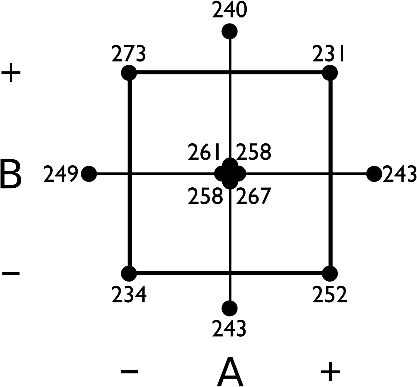
You can check your model with Factorial, the designed-experiments app: generate a central composite design in two factors, with rotatable axial points and 4 center points, type each result against its run, and analyse it with the quadratic model.
If you are using R, you can use the rbind(...) or cbind(...) functions to build up your \(\mathbf{X}\) matrix row-by-row or column-by-column. The equivalent of meshgrid in R is the expand.grid(...) function. See the R code on the course website that shows how to generate surface plots in R.
Question
A full \(2^3\) factorial was run as shown:
Experiment |
A |
B |
C |
|---|---|---|---|
1 |
30% |
232 |
Larry |
2 |
50% |
232 |
Larry |
3 |
30% |
412 |
Larry |
4 |
50% |
412 |
Larry |
5 |
30% |
232 |
Terry |
6 |
50% |
232 |
Terry |
7 |
30% |
412 |
Terry |
8 |
50% |
412 |
Terry |
What would be the D-optimal objective function value for the usual full \(2^3\) factorial model?
If instead experiment 2 was run at (A,B,C) = (45%, 200, Larry), and experiment 3 run at (A, B, C) = (35%, 400, Larry); what would be the D-optimal objective function value?
What is the ratio between the two objective function values?
Solution
The D-optimal objective function is to maximize the determinant of the information matrix, \(\text{det}\left(\mathbf{X}^T\mathbf{X}\right)\).
Since this is a full factorial in 3 factors, with all runs perfectly at the \(-1\) and \(+1\) levels, then the determinant is the product of the diagonal entries and is \(8^8 = 16777216\). In Python, this is
numpy.linalg.det(8 * numpy.eye(8)).Assuming the columns in \(\mathbf{X}\) are in the order of [intercept, A, B, C, AB, AC, BC, ABC], then row 2 in matrix \(\mathbf{X}\) would be \([1, 0.5, -1.356, -1, -0.678, -0.5, 1.356, 0.678]\) and row 3 would be \([1, -0.5, 0.867, -1, -0.433, 0.5, -0.867, 0.433]\)
The determinant with these two rows replaced is now \(6.430 \times 10^6\).
The ratio is \(\frac{6.430 \times 10^6}{16777216} = 0.38\), a fairly large reduction in the objective.
Question
In your start-up company you are investigating treatment options for reducing the contamination level of soil that has been soaked with hydrocarbon products. You have two different heaps of contaminated soil from two different sites. You expect your treatment method to work on any soil type though.
Your limited line of credit allows only 9 experiments, even though you have identified at least 6 factors which you expect to have an effect on the treatment.
Write out the set of experiments that you believe will allow you to learn the most relevant information, given your limited budget. Explain your thinking, and present your answer with 7 columns: 6 columns showing the settings for the 6 factors and one column for the heap from which the test sample should be taken. There should be 9 rows in your table.
What is the projectivity and resolution of your design?
Solution
When given a constraint on the number of experiments, we would like to examine the highest number of factors, but with the lowest tradeoff in the associated resolution.
There are 6 factors to examine. As stated, we would like our treatment method to work on any contaminated soil sample, however we have testing soil only from 2 sites. This is a blocking variable, since we might expect differences due to the site where the soil came from, but we want it to have the least possible effect on our results.
An alternative way to view this problem is to assume that soil is an extra factor in the experiment, but when choosing the generators, we will associate it with the highest level of confounding possible. This latter interpretation makes it easier to use the trade-off table.
Using the trade-off table, and looking down the column with 7 factors, we are constrained to the cell with 8 experiments, since the next cell down has 16 experiments, which is too many. So a \(2^{7-4}_\text{III}\) design would be most appropriate.
We would write out our usual \(2^3\) full factorial, then assign D=AB, E=AC, F=BC and G=ABC. We will let that last factor, the column built from the three-factor interaction ABC, be the heap of soil factor.
We can run a 9th experiment. In this case, I would put all variables at the center point (if they are continuous), and use a 50/50 blend of the two soil samples. Also, I would run this experiment first, to iron out any experimental protocol issues that I did not think of; rather discover them on this first run, which can be discarded in the analysis later on.
Alternatively, if I’m confident with my experimental procedure, I can choose to do experiment 9 last, if at all, as a replicate of any interesting previous experiment that gives an unexpected (good or bad) result.
A table for the experiments would be:
Experiment
A
B
C
D=AB
E=AC
F=BC
G=ABC
1
\(-\)
\(-\)
\(-\)
\(+\)
\(+\)
\(+\)
Heap 1
2
\(+\)
\(-\)
\(-\)
\(-\)
\(-\)
\(+\)
Heap 2
3
\(-\)
\(+\)
\(-\)
\(-\)
\(+\)
\(-\)
Heap 2
4
\(+\)
\(+\)
\(-\)
\(+\)
\(-\)
\(-\)
Heap 1
5
\(-\)
\(-\)
\(+\)
\(+\)
\(-\)
\(-\)
Heap 2
6
\(+\)
\(-\)
\(+\)
\(-\)
\(+\)
\(-\)
Heap 1
7
\(-\)
\(+\)
\(+\)
\(-\)
\(-\)
\(+\)
Heap 1
8
\(+\)
\(+\)
\(+\)
\(+\)
\(+\)
\(+\)
Heap 2
9
0
0
0
0
0
0
50/50
The design has resolution \(R = 3\), from the trade-off table. The projectivity is \(R-1 = 2\).
Question
A factorial experiment was run to investigate the settings that minimize the production of an unwanted side product. The two factors being investigated are called A and B for simplicity, but are:
A = reaction temperature: low level was 420 K, and high level was 440 K
B = amount of surfactant: low level was 10 kg, high level was 12 kg
A full factorial experiment was run, randomly, on the same batch of raw materials, in the same reactor. The system was run on two different days though, and the operator on day 2 was a different person. The recorded amount, in grams, of the side product was:
Experiment |
Run order |
Day |
A |
B |
Side product formed |
|---|---|---|---|---|---|
1 |
2 |
1 |
420 K |
10 kg |
89 g |
2 |
4 |
2 |
440 K |
10 kg |
268 g |
3 |
5 |
2 |
420 K |
12 kg |
179 g |
4 |
3 |
1 |
440 K |
12 kg |
448 g |
5 |
1 |
1 |
430 K |
11 kg |
196 g |
6 |
6 |
2 |
430 K |
11 kg |
215 g |
You can check your analysis with Factorial, the designed-experiments app, which opens these six runs with their results, each on its day.
What might have been the reason(s) for including experiments 5 and 6?
Was the blocking for a potential day-to-day effect implemented correctly in the design? Please show your calculations.
Write out a model that will predict the amount of side product formed. The model should use coded values of A and B. Also write out the \(\mathbf{X}\) matrix and \(\mathbf{y}\) vector that can be used to estimate the model coefficients using the equation \(\mathbf{b} = \left(\mathbf{X'X}\right)^{-1}\mathbf{X'y}\).
Solve for the coefficients of your linear model, either by using \(\mathbf{b} = \left(\mathbf{X'X}\right)^{-1}\mathbf{X'y}\) directly, or by some other method.
Assuming the blocking for the day-to-day effect was implemented correctly, does your model show whether this was an important effect on the response or not? Explain your answer.
You have permission to run two further experiments to find an operating point that reduces the unwanted side product. Where would you place your next two runs, and show how you select these values. Please give your answer in the original units of A and B.
As you move along the response surface, performing new experiments to approach the optimum, how do you know when you are reaching an optimum? How does your experimental strategy change? Please give specific details, and any model equations that might help illustrate your answer.
Solution
Experiments 5 and 6 from the standard order might have been included as baseline experiments, since they appear at the center point for factors A and B.
These two runs give 2 degrees of freedom as well, one of them from the repeat, which estimates the pure error. This helps with estimating confidence intervals on the least squares parameters.
Also, since one of them was performed first, it could have been used to establish the experimental workflow. In other words, the experiment was used to see how to run the experiment the first time. If things go horribly wrong, then this data point can just be discarded. If we had started with a corner of the factorial, we would have had to repeat that experiment if it failed, or if it succeeded, had a duplicate experiment at the one corner but not the others.
Finally, it could also have been used to assess the effect of the operators, since runs 5 and 6 are identical, though in this case runs 5 and 6 are on different days, so it could be the day-to-day being measured here.
Yes. If we consider the day effect to be a new factor, C, then we could treat runs 1 to 4 as a half fraction in 3 factors. The least disruptive generator would be C = AB. Using this we can see that runs 1 and 4 should be run on one day, and runs 2 and 3 on the next day: this is what was done. The center points can be run on either day, and in this case one was run on each day.
Using this generator confounds the interaction effect, AB with the day-to-day (and operator-to-operator) effect. We can never clear up that confounding with this set of experiments.
The model would have the form:
\[y = b_0 + b_A x_A + b_B x_B + b_{AB}x_{AB} + e\]The matrices and vectors to solve this least squares model are:
\[\begin{split}\begin{bmatrix} y_1\\ y_2\\ y_3 \\ y_4 \\ y_5 \\ y_6 \end{bmatrix} &= \begin{bmatrix} 1 & -1 & -1 & +1\\ 1 & +1 & -1 & -1\\ 1 & -1 & +1 & -1\\ 1 & +1 & +1 & +1\\ 1 & 0 & 0 & 0\\ 1 & 0 & 0 & 0\\ \end{bmatrix} \begin{bmatrix} b_0 \\ b_A \\ b_B \\ b_{AB} \end{bmatrix} + \begin{bmatrix} e_1\\ e_2\\ e_3 \\ e_4 \\ e_5 \\ e_6 \end{bmatrix}\\ \begin{bmatrix} 89\\ 268\\ 179\\ 448 \\ 196 \\ 215 \end{bmatrix} &= \begin{bmatrix} 1 & -1 & -1 & +1\\ 1 & +1 & -1 & -1\\ 1 & -1 & +1 & -1\\ 1 & +1 & +1 & +1\\ 1 & 0 & 0 & 0\\ 1 & 0 & 0 & 0\\ \end{bmatrix} \begin{bmatrix} b_0 \\ b_A \\ b_B \\ b_{AB} \end{bmatrix} + \begin{bmatrix} e_1\\ e_2\\ e_3 \\ e_4 \\ e_5 \\ e_6\end{bmatrix}\\ \mathbf{y} &= \mathbf{X} \mathbf{b} + \mathbf{e}\end{split}\]Using the above matrices we can calculate \(\mathbf{b} = \left(\mathbf{X'X}\right)^{-1}\mathbf{X'y}\), even by hand!
\[\begin{split}\mathbf{X'X} & = \begin{bmatrix} 6 & 0 & 0 & 0 \\ 0 & 4 & 0 & 0 \\ 0 & 0 & 4 & 0 \\ 0 & 0 & 0 & 4 \end{bmatrix} \\ \mathbf{X'y} & = \begin{bmatrix} 89 + 268 + 179 + 448 + 196 + 215 \\ -89 + 268 - 179 + 448 \\ -89 - 268 + 179 + 448 \\ +89 - 268 - 179 + 448 \end{bmatrix} = \begin{bmatrix} 1395 \\ 448 \\ 270 \\ 90 \end{bmatrix} \\ \mathbf{b} & = \left(\mathbf{X'X}\right)^{-1}\mathbf{X'y} = \begin{bmatrix} 232.5 \\ 112 \\ 67.5 \\ 22.5 \end{bmatrix}\end{split}\]The above least squares solution shows the two main effects are large: their coefficients are 112 and 67.5 per coded unit. Relative to these two, the interaction term of \(b_{AB} = 22.5\) is small. This implies the day-to-day effect (which is confounded with the operator effect) is small.
A new run in A and B would be at lower values of A and B, since we want to reduce the side product. We will make a move from the baseline point by reducing factor A by 1 unit, and then ratio that with the necessary change in B to go down the direction of steepest descent:
\[\begin{split} \Delta x_A &= -1 \\ \Delta x_{A,\text{actual}} &= -10 \,\text{K} \\ \Delta x_B &= \frac{b_B}{b_A} \Delta x_A = \frac{67.5}{112} \Delta x_A \\ \text{but we know that}\qquad\qquad \Delta x_B &= \frac{\Delta x_{B,\text{actual}}}{\Delta_B / 2} \\ \Delta x_{B,\text{actual}} &= \frac{b_B}{b_A} \Delta x_A \times \Delta_B / 2 \,\,\text{by equating previous 2 lines} \\ \Delta x_{B,\text{actual}} &= \frac{67.5}{112} \times (-1) \times 2 \text{kg} / 2\\ \Delta x_{B,\text{actual}} &= \bf{-0.60}\,\,\text{kg}\\\end{split}\]Note that \(\Delta_B \neq \Delta x_B\). The former is the range for factor B, the latter is the amount by which we change factor B from the baseline. So the new settings for the next experiment would be at:
A =
430 - 10= 420 KB = \(11 - 0.60\) = 10.4 kg
The second run continues one more step along the same direction: A = 410 K and B = \(10.4 - 0.60\) = 9.8 kg.
An optimum is present in a factorial experiment if you notice that:
interaction terms start to become large,
the center point in the factorial has higher/lower values than any of the corner points (remember that with an optimum you are the peak or the valley)
curvature terms, i.e. quadratic terms, in the model are larger than the main effect.
The experimental strategy changes by including axial points into the factorial design, allowing one to calculate the quadratic terms in the model, such as a \(b_{AA} x_A^2\) term for the quadratic effect of factor A.
Question
Adapted from Box, Hunter and Hunter
A liquid polymer formulation is being made that is applied as a polish to wood surfaces. The group responsible for the product have identified 3 elements to the formulation that have an effect of the liquid polish’s final quality attributes (FQAs: this acronym is becoming a standard in most companies these days).
A: amount of reactive monomer in the recipe (10% at the low level and 30% at the high level)
B: the amount of chain length regulator (1% at the low level and 4% at the high level)
C: the type of chain length regulator (regulator P at the \(-\) level or regulator Q at the \(+\) level)
In class we have focused on the case where our \(y\)-variable is continuous, but it could also be descriptive. In this question we also see what happens when we have more than one \(y\)-variable.
\(y_1\) = Milky appearance: either Yes or No
\(y_2\) = Viscous: either Yes or No
\(y_3\) = Yellow colour: either No or Slightly
The following table captures the 8 experiments in standard order, although the experiments were run in a randomized order.
Experiment |
A |
B |
C |
\(y_1\) |
\(y_2\) |
\(y_3\) |
|---|---|---|---|---|---|---|
1 |
\(-\) |
\(-\) |
P |
Yes |
Yes |
No |
2 |
\(+\) |
\(-\) |
P |
No |
Yes |
No |
3 |
\(-\) |
\(+\) |
P |
Yes |
No |
No |
4 |
\(+\) |
\(+\) |
P |
No |
No |
No |
5 |
\(-\) |
\(-\) |
Q |
Yes |
Yes |
No |
6 |
\(+\) |
\(-\) |
Q |
No |
Yes |
Slightly |
7 |
\(-\) |
\(+\) |
Q |
Yes |
No |
No |
8 |
\(+\) |
\(+\) |
Q |
No |
No |
Slightly |
What is the cause of a milky appearance?
What causes a more viscous product?
What is the cause of a slight yellow appearance?
Which conditions would you use to create a product was not milky, was of low viscosity, and had no yellowness?
Which conditions would you use to create a product was not milky, was of low viscosity, and had some yellowness?
Solution
Tables are often frowned on by people, but the reality is they are sometimes one of the best forms of visualizing data. In this example we see:
The milky appearance is caused by low levels of A = amount of reactive monomer (10% in this recipe), since milky appearance is correlated with that column.
A more viscous product is caused by low levels of B = amount of chain length regulator (1% in this recipe), since the change in signs in B match the viscous column.
The yellow appearance is due to an interaction: in this case only when using chain length regulator Q and when using high levels of reactive monomer in the recipe (30%) do we see the yellow appearance.
Such a product can be obtained by using
A = high amount of reactive monomer in the recipe (30%)
B = high amounts of chain length regulator (4%)
C = use chain length regulator P
These correspond to conditions in experiment 4.
Such a product can be obtained by using
A = high amount of reactive monomer in the recipe (30%)
B = high amounts of chain length regulator (4%)
C = use chain length regulator Q
These correspond to conditions in experiment 8.
In all these questions we can conclusively state there is cause and effect, since we see repeated changes in the factors (holding the other variables and disturbances constant) and the corresponding effects in the 3 \(y\)-variables.
Question
Using a \(2^3\) factorial design in 3 variables (A = temperature, B = pH and C = agitation rate), the conversion, \(y\), from a chemical reaction was recorded.
Experiment |
A |
B |
C |
\(y\) |
|---|---|---|---|---|
1 |
\(-\) |
\(-\) |
\(-\) |
72 |
2 |
\(+\) |
\(-\) |
\(-\) |
73 |
3 |
\(-\) |
\(+\) |
\(-\) |
66 |
4 |
\(+\) |
\(+\) |
\(-\) |
87 |
5 |
\(-\) |
\(-\) |
\(+\) |
70 |
6 |
\(+\) |
\(-\) |
\(+\) |
73 |
7 |
\(-\) |
\(+\) |
\(+\) |
67 |
8 |
\(+\) |
\(+\) |
\(+\) |
87 |
A = \(\displaystyle \frac{\text{temperature} - 150\text{°C}}{10\text{°C}}\)
B = \(\displaystyle \frac{\text{pH} - 7.5}{0.5}\)
C = \(\displaystyle \frac{\text{agitation rate} - 50 \text{rpm}}{5 \text{rpm}}\)
You can check your analysis with Factorial, the designed-experiments app, which opens these eight runs with their results.
Show a cube plot for the recorded data.
Estimate the main effects and interactions by hand.
Interpret any results from part 2.
Show that a least squares model for the full factorial agrees with the effects and interactions calculated by hand.
Approximately, at what conditions (given in real-world units), would you run the next experiment to improve conversion. Give your settings in coded units, then unscale and uncenter them to get real-world units.
Solution
A cube plot for the data from these 8 runs is:

The main effects and interactions are:
A effect: There are 4 estimates of \(A = \displaystyle \frac{(73-72) + (87-66) + (73-70) + (87-67)}{4} = \frac{45}{4} = \bf{11.25}\)
B effect: There are 4 estimates of \(B = \displaystyle \frac{(66-72) + (87-73) + (67-70) + (87-73)}{4} = \frac{19}{4} = \bf{4.75}\)
C effect: Again 4 estimates of \(C = \displaystyle \frac{(70-72) + (73-73) + (67-66) + (87-87)}{4} = \frac{-1}{4} = \bf{-0.25}\)
AB interaction: There are 2 estimates of \(AB\). Recall that an interaction is half the difference between the effect of one factor at the high level of the other and its effect at the low level. Consider the change in \(A\) when
\(B_\text{high}\) (at \(C\) high) = 87 - 67 = 20
\(B_\text{low}\) (at \(C\) high) = 73-70 = 3
First estimate = [(20) - (3)]/2 = 8.5
\(B_\text{high}\) (at \(C\) low) = 87 - 66 = 21
\(B_\text{low}\) (at \(C\) low) = 73 - 72 = +1
Second estimate = [(21) - (1)]/2 = 10
Average AB interaction = (8.5 + 10)/2 = 9.25
You can interchange \(A\) and \(B\) and still get the same result.
AC interaction: There are 2 estimates of \(AC\). Consider the change in \(C\) when
\(A_\text{high}\) (at \(B\) high) = 87 - 87 = 0
\(A_\text{low}\) (at \(B\) high) = 67 - 66 = 1
First estimate = [(0) - (+1)]/2 = -0.5
\(A_\text{high}\) (at \(B\) low) = 73 - 73 = 0
\(A_\text{low}\) (at \(B\) low) = 70 - 72 = -2
Second estimate = [(0) - (-2)]/2 = 1
Average AC interaction = (-0.5 + 1)/2 = 0.25
You can interchange \(A\) and \(C\) and still get the same result.
BC interaction: There are 2 estimates of \(BC\): 0 (at high A) and 1.5 (at low A), giving an average BC interaction of 0.75.
ABC interaction: There is only a single estimate:
\(AB\) effect at high \(C\) = 8.5
\(AB\) effect at low \(C\) = 10
\(ABC\) interaction = [(8.5) - (10)] / 2 = -0.75
You can calculate this also by considering the \(AC\) effect at the two levels of \(B\)
Or, you can calculate this by considering the \(BC\) effect at the two levels of \(A\).
All 3 approaches give the same result.
These results show that temperature, A, has by far the greatest effect on the conversion: an increase in conversion of 11.25% when the temperature rises by 20 °C, from 140 °C to 160 °C. The agitation rate, C, has a negligible effect and the effect of pH, B, is between the two: an expected 4.75% increase when the pH rises by 1.0 unit, from 7.0 to 8.0.
There are no interactions involving agitation rate (the BC and AC interactions are both small), so we can safely drop the agitation, factor C, from future consideration in this system.
There is however an interaction between temperature and pH, the AB interaction. This shows that conversion is further increased when both these factors are operated at their high levels.
A least squares model was found by solving for \(\mathbf{b} = \left(\mathbf{X}'\mathbf{X}\right)^{-1}\mathbf{X}'\mathbf{y}\), where
\[\begin{split}\begin{bmatrix} 72\\73\\66\\87\\70\\73\\67\\87 \end{bmatrix} &= \begin{bmatrix} +1 & -1 & -1 & -1 & +1 & +1 & +1 & -1\\ +1 & +1 & -1 & -1 & -1 & -1 & +1 & +1\\ +1 & -1 & +1 & -1 & -1 & +1 & -1 & +1\\ +1 & +1 & +1 & -1 & +1 & -1 & -1 & -1\\ +1 & -1 & -1 & +1 & +1 & -1 & -1 & +1\\ +1 & +1 & -1 & +1 & -1 & +1 & -1 & -1\\ +1 & -1 & +1 & +1 & -1 & -1 & +1 & -1\\ +1 & +1 & +1 & +1 & +1 & +1 & +1 & +1\\ \end{bmatrix} \begin{bmatrix} b_0 \\ b_A \\ b_B \\ b_{C} \\ b_{AB} \\ b_{AC} \\ b_{BC} \\ b_{ABC} \end{bmatrix} \\ \mathbf{y} &= \mathbf{X} \mathbf{b}\end{split}\]which solved for \(\mathbf{b}\) gives the expected model:
\[y = 74.375 + 5.625 x_A + 2.375 x_B -0.125 x_C + 4.625 x_A x_B + 0.125 x_A x_C + 0.375 x_B x_C - 0.375 x_A x_B x_C\]that agrees with the hand-calculations (where the effects are double those from the least squares model).
The experiments can be run at any level of agitation, so it makes sense to use the current midpoint of 50 rpm. We are then left with selecting A and B.
Since we want to increase conversion, we would want to go in any direction that has higher levels of A and B. I would tentatively select A = 1.5 and B as 1.5 in coded units. I used the following code and figure to help my decision (we will see how to select the new point more formally in the section on response surface methods).
Python, 25 lines
import numpy as np
import plotly.graph_objects as go

# The 2^3 design in standard order, with every interaction, and the conversions.
xA = np.array([-1, +1, -1, +1, -1, +1, -1, +1])
xB = np.array([-1, -1, +1, +1, -1, -1, +1, +1])
xC = np.array([-1, -1, -1, -1, +1, +1, +1, +1])
X = np.column_stack([np.ones(8), xA, xB, xC, xA * xB, xA * xC, xB * xC, xA * xB * xC])
conversion = np.array([72, 73, 66, 87, 70, 73, 67, 87])
b = np.linalg.solve(X.T @ X, X.T @ conversion)

# Agitation is held at its midpoint, x_C = 0, which leaves b_0, b_A, b_B and b_AB.
grid = np.linspace(-2, 2, 81)
gA, gB = np.meshgrid(grid, grid)
predicted = b[0] + b[1] * gA + b[2] * gB + b[4] * gA * gB
fig = go.Figure(go.Contour(x=grid, y=grid, z=predicted, contours=dict(showlabels=True)))
fig.add_scatter(x=[-1, 1, -1, 1], y=[-1, -1, 1, 1], mode="markers", name="factorial runs")
fig.add_scatter(x=[1.5], y=[1.5], mode="markers", marker_symbol="star", marker_size=14,
                name="next run")
fig.update_layout(xaxis_title_text="A [temperature, coded]",
                  yaxis_title_text="B [pH, coded]")
fig.show()

print(f"{b[0] + 1.5 * b[1] + 1.5 * b[2] + 1.5 * 1.5 * b[4]:.1f}")
# 96.8

In real-world units these points correspond to:
\(A_\text{actual} = 1.5 \times 10 \text{°C} + 150 \text{°C}\) = 165 °C.
\(B_\text{actual} = 1.5 \times 0.5 + 7.5\) = 8.25 pH units.
The model predicts a conversion of 96.8% there. The point lies outside the cube of the experiments, so this prediction is an extrapolation, which the next run tests.
Question
Why do we block groups of experiments?
Write a \(2^3\) factorial design in two blocks of 4 runs, so that no main effect or 2 factor interaction is confounded with block differences.
Solution
When performing experiments in groups, for example, half the experiments are run on day one and the others on day 2, we must block the experiments we choose to run on each day, to avoid inadvertently introducing a new effect, a day-to-day effect in the model. In other words, we must choose in a careful way the half group of runs we place on day 1 and day 2.
Blocking applies in many other cases: sometimes we have to use two batches of raw materials to do an experiment, because there is not enough for the full factorial. We must block to prevent the effect of raw materials to affect our \(y\)-variable.
Or to run the experiments efficiently in a short time, we choose to do them in parallel in two different reactors. Here we must block against the reactor effect.
For a \(2^3\) system we have factors A, B and C. To keep the main effects and the two-factor interactions clear of the difference between the blocks, we assign the blocks to the highest-order interaction, the ABC interaction.
Writing out the design in standard order:
Experiment
A
B
C
ABC
1
\(-\)
\(-\)
\(-\)
\(-\)
2
\(+\)
\(-\)
\(-\)
\(+\)
3
\(-\)
\(+\)
\(-\)
\(+\)
4
\(+\)
\(+\)
\(-\)
\(-\)
5
\(-\)
\(-\)
\(+\)
\(+\)
6
\(+\)
\(-\)
\(+\)
\(-\)
7
\(-\)
\(+\)
\(+\)
\(-\)
8
\(+\)
\(+\)
\(+\)
\(+\)
This table indicates we should do all experiments in column ABC with a \(-\) in one block, and the experiments with a \(+\) should be done in the second block. In this case no main effect or two-factor interaction is confounded with the block difference; only the ABC interaction is.
Another way you can interpret blocking is as follows. Consider the block to be a new factor in your experiment, call it factor D, where D at the low level corresponds to experiments in the first block, and D at the high level would be experiments in the second block.
But we can only run 8 experiments, so we use the trade-off table, and see the layout that will cause least disruption is to assign D = ABC. This gives the same experimental layout as the table in this solution.
Question
Factors related to the shrinkage of plastic film, produced in an injection molding device, are being investigated. The following factors have been identified by the engineer responsible:
A = mold temperature
B = moisture content
C = holding pressure
D = cavity thickness
E = booster pressure
F = cycle time
G = gate size
Experiment |
A |
B |
C |
D |
E |
F |
G |
\(y\) |
|---|---|---|---|---|---|---|---|---|
1 |
\(-\) |
\(-\) |
\(-\) |
\(+\) |
\(+\) |
\(+\) |
\(-\) |
14.0 |
2 |
\(+\) |
\(-\) |
\(-\) |
\(-\) |
\(-\) |
\(+\) |
\(+\) |
16.8 |
3 |
\(-\) |
\(+\) |
\(-\) |
\(-\) |
\(+\) |
\(-\) |
\(+\) |
15.0 |
4 |
\(+\) |
\(+\) |
\(-\) |
\(+\) |
\(-\) |
\(-\) |
\(-\) |
15.4 |
5 |
\(-\) |
\(-\) |
\(+\) |
\(+\) |
\(-\) |
\(-\) |
\(+\) |
27.6 |
6 |
\(+\) |
\(-\) |
\(+\) |
\(-\) |
\(+\) |
\(-\) |
\(-\) |
24.0 |
7 |
\(-\) |
\(+\) |
\(+\) |
\(-\) |
\(-\) |
\(+\) |
\(-\) |
27.4 |
8 |
\(+\) |
\(+\) |
\(+\) |
\(+\) |
\(+\) |
\(+\) |
\(+\) |
22.6 |
You can check your analysis with Factorial, the designed-experiments app, which opens these eight runs with their results.
You can obtain a copy of this data set if you install the BsMD package in R. Then use the following commands:
S, 5 lines
library(BsMD)
data(BM93.e3.data)

# Use only a subset of the original experiments
X <- BM93.e3.data[1:8, 2:10]
How many experiments would have been required for a full factorial experiment?
What type of fractional factorial is this (i.e. is it a half fraction, quarter fraction …)?
Identify all the generators used to create this design. The trade-off table will help.
Write out the complete defining relationship.
What is the resolution of this design?
Use a least squares approach to calculate a model that fits these 8 experiments.
What effects would you judge to be significant in this system? The engineer will accept your advice and disregard the other factors, and spend the rest of the experimental budget only on the factors deemed significant.
What are these effects aliased with (use your defining relationship to find this).
Why is it necessary to know the confounding pattern for a fractional factorial design.
Solution
There are 7 factors in this experiment, so a full factorial would require \(2^7 = 128\) experiments.
This is a one-sixteenth fraction, 8/128 = 1/16.
Since there are 7 factors in 8 runs, the DOE tradeoff table indicates the possible generators are D = AB, E = AC, F = BC and G = ABC. However, that doesn’t mean the experiments were generated with exactly those factors. For example, these experiments could have interchanged the A and B columns, in which case factors E and F would be different.
However, when checking the columns in our table against these generators we see that the experiments were derived from exactly these same generators. It is customary to record the generators in the form I = …, so our generators are:
I = ABD
I = ACE
I = BCF
I = ABCG.
The defining relationship is the product of all possible generator combinations. Since there are 4 generators, there are \(2^4\) words in the defining relationship. As in the example of a highly fractionated design, the defining relationship is:
I = ABD = ACE = BCF = ABCG = BCDE = ACDF = CDG = ABEF = BEG = AFG = DEF = ADEG = CEFG = BDFG = ABCDEFG
It is a resolution III design, by noting the shortest word in the defining relationship is of length 3 (and verified in the trade-off table).
The least squares model would be found by setting \(-\) = \(-1\) and \(+\) = \(+1\) in the table above as the \(\mathbf{X}\) matrix, and adding an additional column of 1’s to account for the intercept. This gives a total of 8 columns in the matrix. The \(\mathbf{X}^T\mathbf{X}\) will be diagonal, with 8’s on the diagonal. The \(\mathbf{y}\) vector is just the table of results above.
From this we calculate \(\mathbf{b} = \left(\mathbf{X}^T\mathbf{X}\right)^{-1} \mathbf{X}^T\mathbf{y}\) (R code is given at the end).
\[y = 20.35 - 0.65 x_A - 0.25 x_B + 5.05 x_C - 0.45 x_D - 1.45 x_E - 0.15 x_F + 0.15x_G\]Judged with Lenth’s method, only effect C is significant: the pseudo standard error of the seven coefficients is 0.525, so the margin of error is ME = 1.98, which C (5.05) clears and E (-1.45) does not. Effects E and, to a smaller extent, A are the next largest, and an engineer may keep them as candidates for the next experiments.
However, these main effects are aliased with:
C (multiply C by every word in the defining relationship)
CABD = ABCD
CACE = AE
CBCF = BF
CABCG = ABG
CBCDE = BDE
CACDF = ADF
CCDG = DG
CABEF = ABCEF
CBEG = BCEG
CAFG = ACFG
CDEF = CDEF
CADEG = ACDEG
CCEFG = EFG
CBDFG = BCDFG
CABCDEFG = ABDEFG
E (reporting only the 2 factor interactions)
AC
BG
DF
A (reporting only the 2 factor interactions)
BD
CE
FG
It is necessary to know the confounding pattern because it helps to interpret the coefficients. For example, we see that factor C is aliased with the AE interaction, and factors A and E are the next largest effects. We cannot be sure though if that large coefficient for C is due purely to C, or if it is also due to the AE interaction.
The only way we can uncouple that coefficient is by performing additional, foldover experiments.
The R code for this question is given below, and also code to draw the Pareto plot to determine the most important coefficients.
S, 22 lines
A <- B <- C <- c(-1, 1)
d <- expand.grid(A=A, B=B, C=C)
y <- c(14.0, 16.8, 15.0, 15.4, 27.6, 24.0, 27.4, 22.6)
A <- d$A
B <- d$B
C <- d$C
D <- A*B
E <- A*C
F <- B*C
G <- A*B*C
model <- lm(y ~ A + B + C + D + E + F + G)
summary(model)

coeff <- coef(model)[2:length(coef(model))]

# Pareto plot of the absolute coefficients
library(lattice)
bitmap('fractional-factorial-question.png', type="png256",
        width=6, height=6, res=300, pointsize=14)
barchart(sort(abs(coeff)), xlab="Magnitude of effect",
         ylab = "Effect", col=0)
dev.off()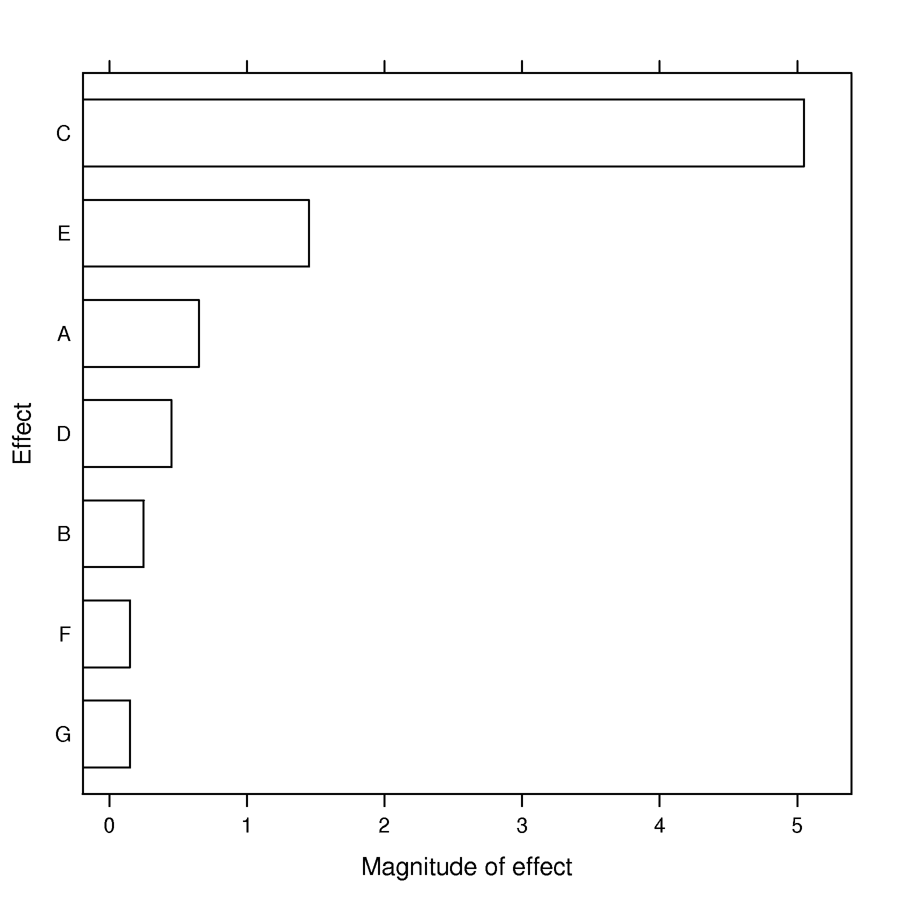
Question
One of the experiment projects investigated by a previous student of this course was understanding effects related to the preparation of uncooked, breaded chicken strips.
The student investigated these 3 factors in a full factorial design \(^\ast\):
D = duration: low level at 15 minutes; and high level = 22 minutes.
R = position of oven rack: low level = use middle rack; high level = use low oven rack (this coding, though unusual, was used because the lower rack applies more heat to the food).
P = preheated oven or not: low level = short preheat (30 seconds); high level = complete preheating.
\(^\ast\) The student actually investigated 4 factors, but found the effect of oven temperature to be negligible!
The response variable was \(y\) = taste, the average of several tasters, with higher values being more desirable.
Experiment
D
R
P
Taste
1
\(-\)
\(-\)
\(-\)
3
2
\(+\)
\(-\)
\(-\)
9
3
\(-\)
\(+\)
\(-\)
3
4
\(+\)
\(+\)
\(-\)
7
5
\(-\)
\(-\)
\(+\)
3
6
\(+\)
\(-\)
\(+\)
10
7
\(-\)
\(+\)
\(+\)
4
8
\(+\)
\(+\)
\(+\)
7
You can check your analysis with Factorial, the designed-experiments app, which opens these eight runs with their results.
A full factorial model, using the usual coding, was calculated from these 8 experiments:
What is the physical interpretation of the \(+2.5 x_\text{D}\) term in the model?
From the above table, at what real-world conditions should you run the system to get the highest taste level?
Does your previous answer match the above model equation? Explain, in particular, how the non-zero two factor interaction term affects taste, and whether the interaction term reinforces the taste response variable, or counteracts it, when the settings you identified in part 2 are used.
If you decided to investigate this system, but only had time to run 4 experiments, write out the fractional factorial table that would use factors D and R as your main effects and confound factor P on the DR interaction.
Now add to your table the response column for taste, extracting the relevant experiments from the above table.
Next, write out the model equation and estimate the 4 model parameters from your reduced set of experiments. Compare and comment on your model coefficients, relative to the full model equation from all 8 experiments.
Solution
A 3.5 minute increase in cooking time, half the range from 15 to 22 minutes, raises the taste by 2.5 units on average.
22 minutes, middle oven rack, with complete preheating.
Yes: the D and P coefficients are positive, so their high levels raise the taste, and the R coefficient is negative, so its low level, the middle rack, raises the taste. The DR interaction has a negative coefficient. This reinforces (improves) the taste, because with D = \(+\) and R = \(-\) the product \(x_\text{D} x_\text{R} = -1\), so the DR term adds to the taste. This term also makes physical sense: if D = \(+\) and R = \(+\), then the taste deteriorates, likely due to the food being overcooked. Similarly, if D = \(-\) and R = \(-\), then the chicken is undercooked.
With P = DR, the four runs are experiments 5, 2, 3 and 8 of the full factorial. In standard order of D and R they have \(y = 3, 9, 3, 7\), and the model is \(y = 5.5 + 2.5 x_D - 0.5 x_R - 0.5 x_P\). The defining relationship I = DRP aliases each coefficient with another term of the full model. The D and R coefficients are unchanged, because their aliases, RP and DP, are zero. The P coefficient is P\(_\text{original}\) + DR\(_\text{original}\) \(= +0.25 - 0.75 = -0.5\), and the intercept is \(b_{0,\text{original}}\) + DRP\(_\text{original}\) \(= 5.75 - 0.25 = 5.5\).
Factorial, the designed-experiments app, opens these four runs with their results.
Question
Your company is developing a microgel-hydrogel composite, used for controlled drug delivery with a magnetic field. A previous employee did the experimental work but she has since left the company. You have been asked to analyze the existing experimental data.
Response variable: \(y\) = sodium fluorescein (SF) released [mg], per gram of gel
The data collected, in the original units:
Experiment
Order
M = microgel weight [%]
H = hydrogel weight [%]
\(y\)
1
4
4
10
119
2
1
8
10
93
3
6
4
16
154
4
3
8
16
89
5
2
6
13
85
6
5
6
13
88
7
9
3.2
13
125
8
7
8.8
13
111
9
10
6
17.2
136
10
8
6
8.8
98
You can check your analysis with Factorial, the designed-experiments app, which opens these ten runs with their results.
What was likely the reason the experimenter added experiments 5 and 6?
Why might the experimenter have added experiments 7, 8, 9 and 10 after the first six? Provide a rough sketch of the design, and all necessary calculations to justify your answer.
What is the name of the type of experimental design chosen by the employee for all 10 experiments in the table?
Using these data, you wish to estimate a nonlinear approximation of the response surface using a model with quadratic terms. Write out the equation of such a model that can be calculated from these 10 experiments (also read the next question).
Write out
the \(\mathbf{X}\) matrix,
the corresponding symbolic entries in \(\mathbf{b}\)
and the \(\mathbf{y}\) vector
that you would use to solve the equation \(\mathbf{b} = \left(\mathbf{X}^T \mathbf{X} \right)^{-1} \mathbf{X}^T \mathbf{y}\) to obtain the parameter estimates of the model you proposed in the previous part. You must use data from all 10 experiments.
How many degrees of freedom will be available to estimate the standard error and confidence intervals?
Solution
These are centerpoint (baseline) runs. They may have been run for some of the following reasons:
To give degrees of freedom for calculating the standard error and then confidence intervals for the slopes.
Trial runs, though they were not done first, so that’s unlikely.
To obtain baseline values for later response surface optimization.
To test the factorial model.
To assess repeatability at the center point.
There might be one or more days that elapsed between the runs, so this assesses the robustness of the model over time
To test for curvature: if the average of the centerpoints, 86.5, is very different from the model’s intercept, \(b_0 = 0.25(119+93+154+89) = 113.75\), as it is in this case, then there is evidence of curvature.
It’s clear that there is evidence of curvature, also, it is feasible the employee was wanting to optimize the response variable. In that case, she would likely use response surface techniques of climbing the path of steepest ascent.
In this model, the presence of curvature at the center point has already been shown. Also a quick calculation from the 4 corner points shows a large two-factor interaction, \(b_{MH} = (119 - 93 - 154 + 89)/4 = -9.75\), compared with the main effects’ coefficients \(b_M = -22.75\) and \(b_H = 7.75\).
Using response surface methods with only the linear terms will be misleading in this case. That’s why the employee decided to add the extra experiments; they are the axial experiments to support quadratic terms.
Central composite design, with the full factorial experiment, in two factors.
\(y = b_0 + b_M x_M + b_H x_H + b_{MH}x_M x_H + b_{MM} x_M^2 + b_{HH}x_H^2\)
In coded units \(x_M = (M - 6)/2\) and \(x_H = (H - 13)/3\), so the four axial runs are at \(\pm 1.4\) coded units. With the columns ordered as the terms of the model above, and the runs in the order of the table:
\[\begin{split}\mathbf{X} = \begin{bmatrix} 1 & -1 & -1 & +1 & 1 & 1 \\ 1 & +1 & -1 & -1 & 1 & 1 \\ 1 & -1 & +1 & -1 & 1 & 1 \\ 1 & +1 & +1 & +1 & 1 & 1 \\ 1 & 0 & 0 & 0 & 0 & 0 \\ 1 & 0 & 0 & 0 & 0 & 0 \\ 1 & -1.4 & 0 & 0 & 1.96 & 0 \\ 1 & +1.4 & 0 & 0 & 1.96 & 0 \\ 1 & 0 & +1.4 & 0 & 0 & 1.96 \\ 1 & 0 & -1.4 & 0 & 0 & 1.96 \end{bmatrix} \qquad \mathbf{b} = \begin{bmatrix} b_0 \\ b_M \\ b_H \\ b_{MH} \\ b_{MM} \\ b_{HH} \end{bmatrix} \qquad \mathbf{y} = \begin{bmatrix} 119 \\ 93 \\ 154 \\ 89 \\ 85 \\ 88 \\ 125 \\ 111 \\ 136 \\ 98 \end{bmatrix}\end{split}\]There are 4 degrees of freedom (10 observations, 6 parameters), one of them pure error, from the two center runs.
Question
Biological drugs are rapidly growing in importance in the treatment of certain diseases, such as cancers and arthritis, since they are designed to target very specific sites in the human body. This can result in treating diseases with minimal side effects. Such drugs differ from traditional drugs in the way they are manufactured – they are produced during the complex reactions that take place in live cell culture. The cells are grown in lab-scale bioreactors, harvested, purified and packaged.
These processes are plagued by low yields which makes these treatments very costly. Your group has run an initial set of experiments to learn more about the system and find better operating conditions to boost the yield. The following factors were chosen in the usual factorial manner:
G = glucose substrate choice: a binary factor, either Gm at the low level code or Gp at the high level.
A = agitation level: low level = 10 rpm and high level = 20 rpm, but can only be set at integer values.
T = growth temperature: 30°C at the low level, or 36°C at the high level, and can only be set at integer values in the future, with a maximum value of 40°C.
C = starting culture concentration: low level = 1100 and high level = 1400, and can only be adjusted in multiples of 50 units and within a range of 1000 to 2000 units.
A fractional factorial in 8 runs at the above settings, created by aliasing C = GAT, gave the following model in coded units:
The aim is to find the next experiment that will improve the yield, measured in milligrams, the most.
What settings might have been used for the baseline conditions for this factorial experiment?
What is the resolution of this design?
Using the method of steepest ascent, state all reasonable assumptions you need to find the experimental conditions for all 4 factors for the next experiment. Give these 4 conditions in both the real-world units, as well as in the usual coded units of the experiment. Note however that your manager has seen that temperature has a strong effect on yield, and he has requested the next experiment be run at 40°C.
Report the expected yield at these proposed experimental conditions.
Solution
Baseline conditions are at G = Gm or Gp (either would work), A at 15 rpm, T at 33 °C, and C at 1250 concentration units.
It is a four factor experiment, with 8 runs. Its defining relationship, I = GATC, has a single word of length 4, so it is a resolution IV design.
We assume that we can ignore all 2fi and 3fi - i.e. that they are small. Specifically, this implies that the 3.5 coefficient is for C and not for the product of \(x_\text{G} x_\text{A} x_\text{T}\)
Fix temperature at 40°C, implying that \(T^\text{(next)} = 40\text{°C}\) and \(x_\text{T}^\text{(next)} = \frac{40-33}{3} = 2.33\).
Factor G must be run at the highest level possible, i.e. G = Gp
Factor A must be run at a lower level, specifically \(\Delta A = -0.25 \times 2.33 = -0.583\), or a deviation of -2.9 rpm from the baseline. Since we have to use integer values, that implies \(A^\text{(next)} = 12\) rpm and \(x_\text{A}^\text{(next)} = \frac{12-15}{5} = -0.6\).
Factor C must be run at a higher level, specifically \(\Delta C = 3.5/4 \times 2.33 = 2.04\), or a deviation of +306 in actual units from the baseline. Since we have to round to the closest 50, that implies \(C^\text{(next)} = 1550\) concentration units and \(x_\text{C}^\text{(next)} = \frac{1550-1250}{150} = +2\).
The predicted yield can be found by substituting the coded values into the model equation, choosing to either use or ignore the small interactions:
With the interactions:
\[\begin{split}\begin{array}{rcl} y &=& 24 + 3 (+1) - 1.0 (-0.6) + 4.0 (2.33) - 0.2 (+1)(-0.6) - 0.79 (+1)(2.33) - 0.25(-0.6)(2.33) + 3.5 (+2) \\ y &=& {\bf 42.5} \end{array}\end{split}\]In this resolution IV design each two-factor interaction is aliased with another: GA with TC, GT with AC, and AT with GC. The prediction with interactions is therefore not unique: attributing the three coefficients to TC, AC and GC instead gives 43.4.
Without interactions:
\[y = 24 + 3 (+1) - 1.0 (-0.6) + 4.0 (2.33) + 3.5 (+2) = 43.9\]
Question
A coating process has been studied with a central composite design in two factors, both coded to the usual \(-1\) to \(+1\) range: \(x_1\) is the line speed and \(x_2\) is the drying temperature. Two responses were measured on every run, and the following models were fitted:
\(\hat{y}_1\) = coating yield [%] = \(80 + 6 x_1 + 2 x_2\)
\(\hat{y}_2\) = unit cost [$/kg] = \(50 + 8 x_1 - 3 x_2\)
The yield must be at least 84%, and the unit cost must be no more than $56/kg.
Where in the region is the yield highest, and where is the cost lowest? Show that no single setting achieves both.
Two settings are proposed: \(R\) at \((x_1, x_2) = (+0.5, +1)\) and \(S\) at \((x_1, x_2) = (+1, +1)\). Does each one meet both requirements? What does the sweet spot tell you about which to prefer?
Using a desirability ramp that runs from 84% to 90% for the yield, and from $56/kg down to $44/kg for the cost, calculate the individual desirabilities and the overall desirability at \(R\) and at \(S\). Which setting does this prefer, and why does it differ from what the yield alone suggests?
A third setting \(P\) at \((x_1, x_2) = (+1, 0)\) gives a yield of 86% and a cost of $58/kg. Calculate its overall desirability and explain the result.
Solution
Both models are planar, so each response is extreme at a corner of the region. The yield rises with both factors, so it is highest at \((+1, +1)\), giving \(80 + 6 + 2 = 88\%\). The cost falls as \(x_1\) decreases and as \(x_2\) increases, so it is lowest at \((-1, +1)\), giving \(50 - 8 - 3 = 39\) $/kg. These are different corners: at \((+1, +1)\) the cost is \(50 + 8 - 3 = 55\) $/kg, and at \((-1, +1)\) the yield is only \(80 - 6 + 2 = 76\%\), which fails the 84% requirement. Line speed helps the yield and hurts the cost, so no setting can be best for both.
At \(R = (+0.5, +1)\): yield \(= 80 + 3 + 2 = 85\%\) and cost \(= 50 + 4 - 3 = 51\) $/kg. At \(S = (+1, +1)\): yield \(= 88\%\) and cost \(= 55\) $/kg. Both settings meet both requirements, so both lie inside the sweet spot. That is all the sweet spot has to say: it marks out the acceptable region but does not rank the settings within it.
The yield is being maximized, so \(d_1 = (y_1 - 84)/(90 - 84)\). The cost is being minimized, so \(d_2 = (56 - y_2)/(56 - 44)\). The overall desirability is the geometric mean, \(D = \sqrt{d_1 d_2}\), with equal importance on each.
At \(R\): \(d_1 = 1/6 = 0.167\) and \(d_2 = 5/12 = 0.417\), so \(D = \sqrt{(1/6)(5/12)} = 0.264\).
At \(S\): \(d_1 = 4/6 = 0.667\) and \(d_2 = 1/12 = 0.083\), so \(D = \sqrt{(4/6)(1/12)} = 0.236\).
Desirability prefers \(R\), even though \(S\) has the higher yield. The cost at \(S\), $55/kg, is only $1/kg inside its limit, which leaves \(d_2\) very small. The geometric mean penalises that imbalance: a setting that is barely acceptable on one response scores poorly overall however well it does on the other. Note that this ranking follows from the ramps chosen; different limits would give a different answer, which is why the ramps have to be stated.
At \(P\) the cost of $58/kg is above the $56/kg limit, so \(d_2 = 0\) and therefore \(D = \sqrt{d_1 \times 0} = 0\), whatever the yield does. \(P\) lies outside the sweet spot, and the overall desirability records that as a zero rather than as a low score. This is the property that makes the geometric mean the usual choice here: an arithmetic mean would have given \(P\) a score of \((0.333 + 0)/2 = 0.167\), letting a good yield partly excuse a product that cannot be sold at that cost.