
 Download PDF of entire book
5.8.6. Assessing significance of main effects and interactions
When there are no replicate points, then the number of parameters to estimate from a full factorial is \(2^k\) from the \(2^k\) observations. There are no degrees of freedom left to calculate the standard error or the confidence intervals for the main effects and interaction terms.
The standard error can be estimated if complete replicates are available. However, a complete replicate is onerous, because a complete replicate implies the entire experiment is repeated: system setup, running the experiment and measuring the result. Taking two samples from one actual experiment and measuring \(y\) twice is not a true replicate. That is only an estimate of the measurement error and analytical error.
Furthermore, there are better ways to spend our experimental budget than running complete replicate experiments – see the section on screening designs later on. Only later in the overall experimental procedure should we run replicate experiments as a verification step and to assess the statistical significance of effects.
There are three ways to judge whether a main effect or interaction is significant. The first two need no replicate runs: a Pareto plot ranks the effects, and Lenth’s method, together with the half-normal plot, adds an objective cutoff to that ranking. The third uses the standard error, and becomes available once replicate runs, center points, or an external estimate of the noise supply some degrees of freedom.
5.8.6.1. Pareto plot
Note
The Pareto plot ranks the effects but leaves the cutoff to the eye; the next section adds an objective one. It is only meaningful when the factors are centered and scaled, so that the coefficients are directly comparable.
A full factorial with \(2^k\) experiments has \(2^k\) parameters to estimate. Once these parameters have been calculated, for example, by using a least squares model, then plot as shown the absolute value of the model coefficients in sorted order, from largest magnitude to smallest, ignoring the intercept term. Significant coefficients are established by visual judgement – establishing a visual cutoff by contrasting the small coefficients to the larger ones.
The example below is from a \(2^4\) full factorial (four factors, sixteen runs) where the results for \(y\) in standard order were \(y = \left[45,71,48,65,68,60,80,65,43,100,45,104,75,86,70,96 \right]\). The code fits the sixteen-parameter model by least squares and plots the sorted magnitudes of the fifteen effects.
Python, 36 lines
import itertools
import numpy as np
import plotly.graph_objects as go

# Full 2^4 factorial in standard (Yates) order: factor A alternates fastest.
levels = [-1, 1]
design = np.array(list(itertools.product(levels, levels, levels, levels)))[:, ::-1]
y = np.array([45, 71, 48, 65, 68, 60, 80, 65,
              43, 100, 45, 104, 75, 86, 70, 96])

# Build every main effect and interaction column, then fit by least squares.
names = ["A", "B", "C", "D"]
factor = {name: design[:, i] for i, name in enumerate(names)}
terms = {}
for order in range(1, 5):
    for combo in itertools.combinations(names, order):
        column = np.ones(16)
        for f in combo:
            column = column * factor[f]
        terms["".join(combo)] = column

X = np.column_stack([np.ones(16)] + list(terms.values()))
b = np.linalg.solve(X.T @ X, X.T @ y)   # X is orthogonal, so this is exact
effects = dict(zip(terms.keys(), b[1:]))  # drop the intercept

# Pareto plot: absolute effects, largest bar at the top. Colour each bar by the
# sign of its effect, using the colourblind-safe Okabe-Ito pair: orange for a
# positive effect, blue for a negative one.
ordered = sorted(effects, key=lambda name: abs(effects[name]))
orange, blue = "#E69F00", "#0072B2"
colours = [orange if effects[name] > 0 else blue for name in ordered]
fig = go.Figure(go.Bar(x=[abs(effects[name]) for name in ordered],
                       y=ordered, orientation="h", marker_color=colours))
fig.update_layout(xaxis_title_text="|effect|", yaxis_title_text="Term",
                  showlegend=False)
fig.show()
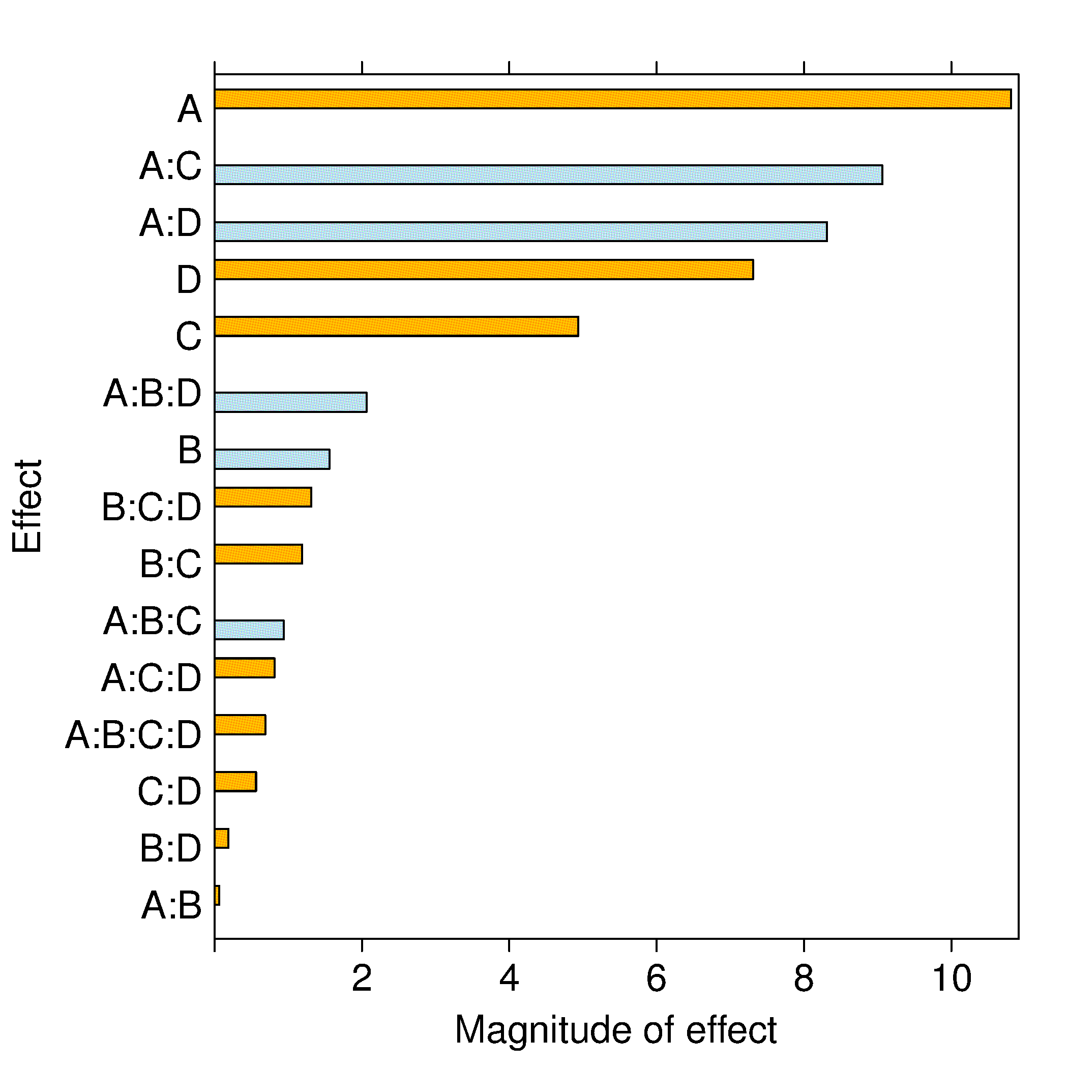
Each bar is coloured by the sign of its effect: orange for a positive coefficient and blue for a negative one (the colourblind-safe Okabe-Ito pair), so the bar length shows the magnitude while its colour shows the direction. The two dashed and dotted vertical lines in the figure are the Lenth margins of error introduced in the next section; they, not the colour, mark where significance begins.
We would interpret that factors A, C and D, as well as the interactions of AC and AD, have a significant and causal effect on the response variable, \(y\). The main effect of B on the response \(y\) is small, at least over the range that B was used in the experiment. Factor B can be omitted from future experimentation in this region, though it might be necessary to include it again if the system is operated at a very different point.
The reason why we can compare the coefficients this way, which is not normally the case with least squares models, is that we have both centered and scaled the factor variables. If the centering is at typical baseline operation, and the range spanned by each factor is that expected over the typical operating range, then we can fairly compare each coefficient in the bar plot. Each bar represents the influence of that term on \(y\) for a one-unit change in the factor, that is, a change over half its operating range.
If the factors are not scaled appropriately, then this method will be error prone. The effects themselves are always estimated by least squares; what the Pareto plot adds is a ranking. For highly fractionated and saturated designs, where there are no degrees of freedom for a standard error, the Pareto plot and the Lenth’s-method cutoff of the next section are the tools available.
5.8.6.2. Lenth’s method and the half-normal plot: an objective cutoff
The Pareto plot ranks the effects but leaves the cutoff to the eye. When the design is unreplicated, so there are no degrees of freedom for a standard error, we can still place an objective cutoff by using the idea of effect sparsity: in most systems only a few of the many effects are real, and the rest scatter around zero at the size of the experimental noise. Those many near-zero effects can therefore be used to estimate the noise, and any effect standing well clear of that noise is judged significant.
Lenth’s method turns this into a number. Work with the estimated effects, here the model coefficients \(c_1, c_2, \ldots, c_m\), excluding the intercept (for a \(2^4\) factorial \(m = 15\)). The steps are:
The pseudo standard error (PSE) is a robust estimate of the standard error of an effect. The first median sets a rough scale, \(s_0\); the second median is then taken only over the effects small enough (within \(2.5\, s_0\)) to be plausibly noise, so that a few large, real effects cannot inflate it. The margin of error (ME) is the individual 95% cutoff: an effect whose magnitude exceeds the ME is significant on its own. The simultaneous margin of error (SME) allows for testing all \(m\) effects at once. Its \(t\)-value is taken at \(\gamma\), so that each noise effect stays below the SME with probability \(0.95^{1/m}\), and all \(m\) of them together, were they independent, with probability 0.95. It is the stricter cutoff to use when scanning many effects at once. Lenth’s rule sets the degrees of freedom for the \(t\)-value to \(d = m/3\).
Applying this to the \(2^4\) example above, reusing the effects computed for the Pareto plot:
Python, 17 lines
import numpy as np
from scipy import stats

coeffs = np.array(list(effects.values()))
m = len(coeffs)                                       # 15 effects
abs_c = np.abs(coeffs)
s0 = 1.5 * np.median(abs_c)
pse = 1.5 * np.median(abs_c[abs_c < 2.5 * s0])
d = m / 3
ME = stats.t.ppf(0.975, d) * pse
SME = stats.t.ppf((1 + 0.95 ** (1 / m)) / 2, d) * pse
print(f"PSE = {pse:.2f}, ME = {ME:.2f}, SME = {SME:.2f}")
# PSE = 1.31, ME = 3.37, SME = 6.85

print(sorted((k for k in effects if abs(effects[k]) > ME),
             key=lambda k: -abs(effects[k])))
# ['A', 'AC', 'AD', 'D', 'C']
The pseudo standard error is \(\text{PSE} = 1.31\), so the margin of error is \(\text{ME} = 3.37\). Five effects exceed it, A, C, D, AC and AD, exactly the five the eye picked from the Pareto plot. The simultaneous margin of error is \(\text{SME} = 6.85\): A, D, AC and AD clear even that stricter bar, while C (\(|c_C| = 4.9\)) sits between the two margins, significant individually but not once we allow for having scanned all fifteen effects.
The half-normal plot shows the same judgement graphically, and is the plot JMP, Minitab and Stat-Ease draw for unreplicated designs. Order the effects by absolute value and plot them against the quantiles of the half-normal distribution at the plotting positions \((i - 0.5)/m\). Noise effects fall along a straight line through the origin; the real effects break away to the upper right.
Python, 10 lines
import plotly.graph_objects as go

ordered = sorted(effects, key=lambda k: abs(effects[k]))
absv = np.array([abs(effects[k]) for k in ordered])
quantiles = stats.halfnorm.ppf((np.arange(1, m + 1) - 0.5) / m)
fig = go.Figure(go.Scatter(x=quantiles, y=absv, mode="markers+text",
                           text=ordered, textposition="top left"))
fig.update_layout(xaxis_title_text="Half-normal quantile",
                  yaxis_title_text="|effect|", showlegend=False)
fig.show()
Running the block draws the half-normal plot: the ten noise effects sit on a line through the origin, and A, C, D, AC and AD stand clear of it.
The same result is available directly from process_improve. Note that analyze_experiment reports effects on the high-to-low scale (twice the model coefficient, the Box, Hunter and Hunter convention), so its PSE, ME and SME come out at twice the values above; the significance decision is identical, because both the effects and the cutoff double.
Python, 14 lines
import pandas as pd
from process_improve.experiments.analysis import analyze_experiment
from process_improve.experiments.visualization.plots.registry import create_plot

frame = pd.DataFrame(design, columns=names)
frame["y"] = y
res = analyze_experiment(frame, response_column="y", model="A*B*C*D",
                         analysis_type=["effects", "lenth_method"])
lenth = res["lenth_method"]
print(f"PSE = {lenth['PSE']:.3f}, ME = {lenth['ME']:.3f}, SME = {lenth['SME']:.3f}")
# PSE = 2.625, ME = 6.748, SME = 13.699

create_plot("pareto", analysis_results=res).to_plotly()  # Pareto with ME and SME lines
create_plot("half_normal", analysis_results=res).to_plotly()  # the half-normal plot
The pseudo-standard-error cutoff is from Lenth (1989), “Quick and Easy Analysis of Unreplicated Factorials”, Technometrics, 31, 469-473. The half-normal plot of effects is due to Daniel (1959), “Use of Half-Normal Plots in Interpreting Factorial Two-Level Experiments”, Technometrics, 1, 311-341.
5.8.6.3. Standard error: from replicate runs or from an external dataset
Note
It is often better to spend your experimental budget screening for additional factors rather than replicating experiments.
If a duplicate run exists at every combination of the factorial, then the standard error can be estimated directly:
Let \(y_{i,1}\) and \(y_{i,2}\) be the two response values for each of the \(i^\text{th}\) runs, where \(i=1, 2, \ldots, 2^k\).
The mean response for the \(i^\text{th}\) run is \(\overline{y}_i = 0.5\,y_{i,1} + 0.5\,y_{i,2}\).
Denote the difference between them as \(d_i = y_{i,2} - y_{i,1}\) (the sign does not matter).
Each pair gives a variance estimate on a single degree of freedom, \(s_i^2 = \dfrac{(y_{i,1} - \overline{y}_i)^2 + (y_{i,2} - \overline{y}_i)^2}{1} = \dfrac{d_i^2}{2}\).
Pooling these \(2^k\) single-degree-of-freedom estimates means averaging them, giving \(\widehat{\sigma}^2 = S_E^2 = \dfrac{1}{2^k}\displaystyle\sum_{i=1}^{2^k}{s_i^2} = \dfrac{1}{2^{k+1}}\displaystyle\sum_{i=1}^{2^k}{d_i^2}\), on \(2^k\) degrees of freedom.
Each coefficient’s ratio \(b_i / S_E(b_i)\) is then \(t\)-distributed on those \(2^k\) degrees of freedom, which is what makes the confidence interval and significance test possible.
The standard error can be found in a similar way if more than one duplicate run is performed. Note that a full replicate is expensive: as discussed in the screening designs section, it is often more productive to spend those extra runs on additional factors than on repeating existing runs.
If there are more experiments than parameters to be estimated, then we have extra degrees of freedom. Having degrees of freedom implies we can calculate the standard error, \(S_E\). Once \(S_E\) has been found, we can also calculate the standard error for each model coefficient, and then confidence intervals can be constructed for each main effect and interaction. And because the model matrix is orthogonal, the confidence interval for each effect is independent of the other. This is because the variance-covariance matrix of the estimates is \(\mathcal{V}\left(\mathbf{b}\right) = \left(\mathbf{X}^T\mathbf{X}\right)^{-1}S_E^2\), and the off-diagonal elements in \(\mathbf{X}^T\mathbf{X}\) are zero, so the estimates are uncorrelated. The confidence interval for each coefficient is then \(b_i \pm c_t \sqrt{\mathcal{V}(b_i)}\).
For an experiment with \(n\) runs, and where we have coded our \(\mathbf{X}\) matrix to contain \(-1\) and \(+1\) elements, and when the \(\mathbf{X}\) matrix is orthogonal, the standard error for coefficient \(b_i\) is \(S_E(b_i) = \sqrt{\mathcal{V}\left(b_i\right)} = \sqrt{\dfrac{S_E^2}{\sum{x_i^2}}}\). Some examples:
A \(2^3\) factorial where every combination has been repeated will have \(n=16\) runs, so the standard error for each coefficient will be the same, at \(S_E(b_i) = \sqrt{\dfrac{S_E^2}{16}} = \dfrac{S_E}{4}\).
A \(2^3\) factorial with three additional runs at the center point would have the following least squares representation:
\[\begin{split}\mathbf{y} &= \mathbf{X} \mathbf{b} + \mathbf{e}\\ \begin{bmatrix} y_1\\ y_2\\ y_3 \\ y_4 \\ y_5 \\ y_6 \\ y_7 \\ y_8 \\ y_{c,1} \\ y_{c,2} \\ y_{c,3}\end{bmatrix} &= \begin{bmatrix} 1 & A_{-} & B_{-} & C_{-} & A_{-}B_{-} & A_{-}C_{-} & B_{-}C_{-} & A_{-}B_{-}C_{-}\\ 1 & A_{+} & B_{-} & C_{-} & A_{+}B_{-} & A_{+}C_{-} & B_{-}C_{-} & A_{+}B_{-}C_{-}\\ 1 & A_{-} & B_{+} & C_{-} & A_{-}B_{+} & A_{-}C_{-} & B_{+}C_{-} & A_{-}B_{+}C_{-}\\ 1 & A_{+} & B_{+} & C_{-} & A_{+}B_{+} & A_{+}C_{-} & B_{+}C_{-} & A_{+}B_{+}C_{-}\\ 1 & A_{-} & B_{-} & C_{+} & A_{-}B_{-} & A_{-}C_{+} & B_{-}C_{+} & A_{-}B_{-}C_{+}\\ 1 & A_{+} & B_{-} & C_{+} & A_{+}B_{-} & A_{+}C_{+} & B_{-}C_{+} & A_{+}B_{-}C_{+}\\ 1 & A_{-} & B_{+} & C_{+} & A_{-}B_{+} & A_{-}C_{+} & B_{+}C_{+} & A_{-}B_{+}C_{+}\\ 1 & A_{+} & B_{+} & C_{+} & A_{+}B_{+} & A_{+}C_{+} & B_{+}C_{+} & A_{+}B_{+}C_{+}\\ 1 & 0 & 0 & 0 & 0 & 0 & 0 & 0 \\ 1 & 0 & 0 & 0 & 0 & 0 & 0 & 0 \\ 1 & 0 & 0 & 0 & 0 & 0 & 0 & 0 \end{bmatrix} \begin{bmatrix} b_0 \\ b_A \\ b_B \\ b_{C} \\ b_{AB} \\ b_{AC} \\ b_{BC} \\ b_{ABC} \end{bmatrix} + \begin{bmatrix} e_1\\ e_2\\ e_3 \\ e_4 \\ e_5 \\ e_6 \\ e_7 \\ e_8 \\ e_{c,1} \\ e_{c,2} \\ e_{c,3} \end{bmatrix}\\\end{split}\]And substituting in the values, using vector shortcut notation for \(\mathbf{y}\) and \(\mathbf{e}\):
\[\begin{split}\mathbf{y} &= \begin{bmatrix} 1 & -1 & -1 & -1 & +1 & +1 & +1 & -1\\ 1 & +1 & -1 & -1 & -1 & -1 & +1 & +1\\ 1 & -1 & +1 & -1 & -1 & +1 & -1 & +1\\ 1 & +1 & +1 & -1 & +1 & -1 & -1 & -1\\ 1 & -1 & -1 & +1 & +1 & -1 & -1 & +1\\ 1 & +1 & -1 & +1 & -1 & +1 & -1 & -1\\ 1 & -1 & +1 & +1 & -1 & -1 & +1 & -1\\ 1 & +1 & +1 & +1 & +1 & +1 & +1 & +1\\ 1 & 0 & 0 & 0 & 0 & 0 & 0 & 0\\ 1 & 0 & 0 & 0 & 0 & 0 & 0 & 0\\ 1 & 0 & 0 & 0 & 0 & 0 & 0 & 0 \end{bmatrix} \begin{bmatrix} b_0 \\ b_A \\ b_B \\ b_{C} \\ b_{AB} \\ b_{AC} \\ b_{BC} \\ b_{ABC} \end{bmatrix} + \mathbf{e}\end{split}\]Note that the center point runs do not change the orthogonality of \(\mathbf{X}\) (verify this by writing out and computing the \(\mathbf{X}^T\mathbf{X}\) matrix and observing that all off-diagonal entries are zeros). However, as we expect after having studied the section on least squares modelling, additional runs decrease the variance of the model parameters, \(\mathcal{V}(\mathbf{b})\). In this case, there are \(n=2^3+3 = 11\) runs, so the standard error is decreased to \(S_E^2 = \dfrac{\mathbf{e}^T\mathbf{e}}{11 - 8}\). However, the center points do not further reduce the variance of the parameters in \(\sqrt{\dfrac{S_E^2}{\sum{x_i^2}}}\), because the denominator is still \(2^k\) (except for the intercept term, whose variance is reduced by the center points).
Once we obtain the standard error for our system and calculate the variance of the parameters, we can multiply it by the critical \(t\)-value at the desired confidence level in order to calculate the confidence limit. However, it is customary to just report the standard error next to the coefficients, so that users can apply their own level of confidence. For example,
\[\begin{split}\text{Temperature effect}, b_T &= 11.5 \pm 0.707\\ \text{Catalyst effect}, b_K &= 1.1 \pm 0.707\end{split}\]
Even though the confidence interval of the temperature effect would be \(11.5 - c_t \times 0.707 \leq \beta_T \leq 11.5 + c_t \times 0.707\), it is clear that at the 95% confidence level, the above representation shows the temperature effect is significant, while the catalyst effect is not (\(c_t \approx 2\)).
5.8.6.4. Refitting the model after removing nonsignificant effects
After having established which effects are significant, we can exclude the nonsignificant effects and increase the degrees of freedom. (We do not have to recalculate the model parameters – why?) The residuals will be nonzero now, so we can then estimate the standard error and apply all the tools from least squares modelling to assess the residuals. Plots of the residuals in experimental order, against fitted values, q-q plots and all the other assessment tools from earlier are used, as usual.
As an example, consider a \(2^4\) factorial (16 runs) where the response values in standard order were \(y = [71, 61, 90, 82, 68, 61, 87, 80, 61, 50, 89, 83, 59, 51, 85, 78]\). Assessing the 15 effects with a Pareto plot, or with Lenth’s method, identifies A, B, D and BD as the significant ones. Now, omitting the nonsignificant effects, there are only five parameters to estimate, including the intercept, so the standard error is \(S_E^2 = \dfrac{39}{16-5} = 3.55\), with 11 degrees of freedom. The \(S_E(b_i)\) value for all coefficients, except the intercept, is \(\sqrt{\dfrac{S_E^2}{16}} = 0.471\), and the critical \(t\)-value at the 95% level is qt(0.975, df=11) = 2.2. So the confidence intervals can be calculated to confirm that these are indeed significant effects. The same yardstick, \(2.2 \times 0.471 = 1.04\), is also exceeded by one of the omitted effects, \(b_C = -1.125\).
Factorial, the designed-experiments app, opens these 16 runs with their results, fitted with only A, B, D and BD.
There is some circular reasoning here: postulate that one or more effects are zero and increase the degrees of freedom by removing those parameters in order to confirm the remaining effects are significant. Some general advice is to first exclude effects that are definitely small, and then retain medium-size effects in the model until you can confirm they are not significant.
5.8.6.5. Variance of estimates from the COST approach versus the factorial approach
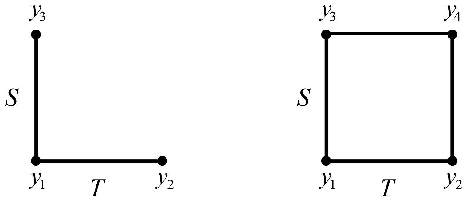
Finally, we end this section on factorials by illustrating their efficiency. Contrast the two cases: COST and the full factorial approach. For this analysis we define the main effect simply as the difference between the high and low values (normally we divide through by 2, but the results still hold). Define the variance of the measured \(y\) value as \(\sigma_y^2\).
COST approach |
Factorial approach |
|---|---|
The main effect of \(T\) is \(b_T = y_2 - y_1\). |
The main effect is \(b_T = 0.5(y_2 - y_1) + 0.5(y_4 - y_3)\). |
The variance is \(\mathcal{V}(b_T) = \sigma_y^2 + \sigma_y^2\). |
The variance is \(\mathcal{V}(b_T) = 0.25(\sigma_y^2 + \sigma_y^2) + 0.25(\sigma_y^2 + \sigma_y^2)\). |
So \(\mathcal{V}(b_T) = 2\sigma_y^2\). |
And \(\mathcal{V}(b_T) = \sigma_y^2\). |
The factorial uses all four runs to estimate \(b_T\), whereas the COST comparison uses only two, so part of the variance reduction is simply the extra runs. The point is that those same four runs also estimate \(b_S\) and the interaction \(b_{TS}\) at no additional cost, whereas the COST approach cannot estimate the effect of interactions at all. Interactions are important, especially as systems approach optima that lie on ridges (see the contour plots earlier in this section for an example).
Factorial designs make each experimental observation work twice.