2.9. The t-distribution¶

Suppose we have a quantity of interest from a process, such as the daily profit. In the preceding section we started to answer the useful and important question:

What is the range within which the true average value lies? E.g. the range for the true, but unknown, daily profit.

But we got stuck, because the lower and upper bounds we calculated for the true average, \(\mu\) were a function of the unknown population standard deviation, \(\sigma\). Repeating the prior equation for confidence interval where we know the variance:

\[\begin{split}\begin{array}{rcccl} - c_n &\leq& \displaystyle \frac{\overline{x} - \mu}{\sigma/\sqrt{n}} &\leq & +c_n\\ \overline{x} - c_n \dfrac{\sigma}{\sqrt{n}} &\leq& \mu &\leq& \overline{x} + c_n\dfrac{\sigma}{\sqrt{n}} \\ \text{LB} &\leq& \mu &\leq& \text{UB} \end{array}\end{split}\]

which we derived by using the fact that \(\dfrac{\overline{x} - \mu}{\sigma/\sqrt{n}}\) is normally distributed.

An obvious way out of our dilemma is to replace \(\sigma\) by the sample standard deviation, \(s\), which is exactly what we will do, however, the quantity \(\frac{\overline{x} - \mu}{s/\sqrt{n}}\) is not normally distributed, but is \(t\)-distributed. Before we look at the details, it is helpful to see how similar in appearance the \(t\) and normal distribution are: the \(t\)-distribution peaks slightly lower than the normal distribution, but it has broader tails. The total area under both curves illustrated here is 1.0.

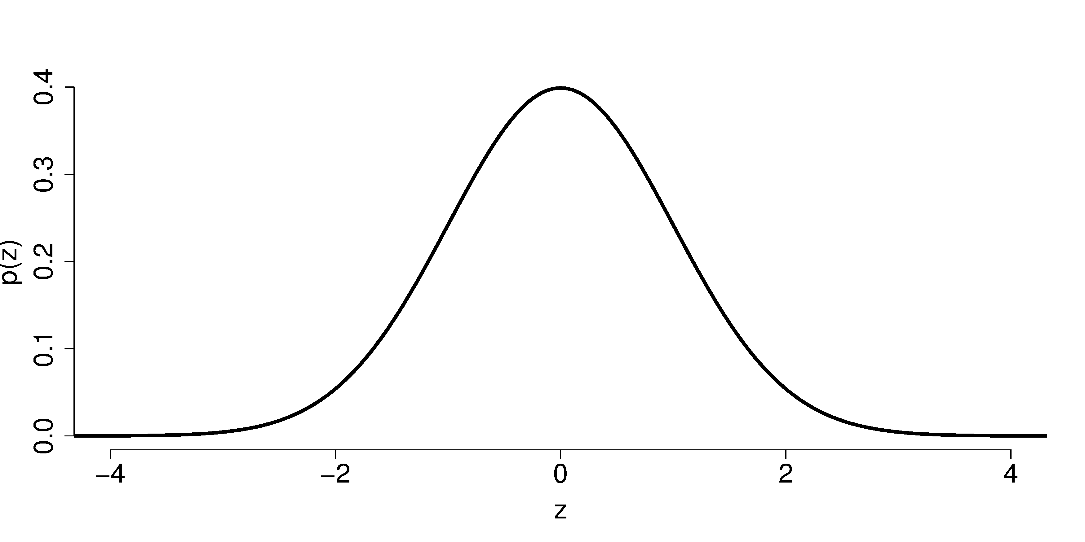
There is one other requirement we have to ensure in order to use the \(t\)-distribution: the values that we sample, \(x_i\) must come from a normal distribution (carefully note that in the previous section we didn’t have this restriction!). Fortunately it is easy to check this requirement: just use the q-q plot method described earlier. Another requirement, which we had before, was that we must be sure these measurements, \(x_i\), are independent.

../_images/t-distribution-derivation.png

So given our \(n\) samples, which are independent, and from a normal distribution, we can now say:

(1)¶\[\frac{\overline{x} - \mu}{s/\sqrt{n}} \sim t_{n-1}\]

Compare this to the previous case where our \(n\) samples are independent, and we happen to know, by some unusual way, what the population standard deviation is, \(\sigma\):

\[\frac{\overline{x} - \mu}{\sigma/\sqrt{n}} \sim \mathcal{N} \left(0, 1\right)\]

So the more practical and useful case where \(\dfrac{\overline{x} - \mu}{s/\sqrt{n}} \sim t_{n-1}\) can now be used to construct an interval for \(\mu\). This standardized quantity follows the \(t\)-distribution with \(n-1\) degrees of freedom, where the degrees of freedom come from calculating the estimated standard deviation, \(s\).

It helps to be explicit about the notation, because two different distributions are now in play. When the population standard deviation \(\sigma\) is known, the standardized quantity \(\dfrac{\overline{x} - \mu}{\sigma/\sqrt{n}}\) follows the standard normal distribution, and we called it a \(z\)-deviate. When \(\sigma\) is replaced by its estimate \(s\), the standardized quantity \(\dfrac{\overline{x} - \mu}{s/\sqrt{n}}\) follows the \(t\)-distribution instead; some texts write it as a \(t\)-value. This book keeps calling any such standardized quantity a \(z\)-deviate, but which distribution applies depends on whether the standard deviation is known (the normal) or estimated (the \(t\)-distribution).

Note that this standardized quantity only requires we know the population mean (\(\mu\)), not the population standard deviation; we use our estimate \(s/\sqrt{n}\) of the standard error in place of the population value.

We will come back to (1) in a minute; let’s first look at how we can calculate values from the \(t\)-distribution in computer software.

2.9.1. Calculating the t-distribution¶

In R we use the function dt(x=..., df=...) to give us the values of the probability density values, \(p(x)\), of the \(t\)-distribution (compare this to the dnorm(x, mean=..., sd=...) function for the normal distribution).

Python, 18 lines

from scipy.stats import norm, t

x = 0.0

# Recall, for the normal distribution:
norm.pdf(x, loc=0, scale=1)   # 0.3989423

# For the t-distribution we don't have
# a sigma, but we do need to say how
# many degrees of freedom we have:

dof = 8
t.pdf(x, df=dof)              # 0.386699

# Shows that the t-distribution has a
# lower peak than the normal distribution.
# Try it again, but with fewer and
# greater degrees of freedom (`dof`).

R, 16 lines

x = 0.0

# Recall, for the normal distribution:
dnorm(x, mean=0, sd=1)    # 0.3989423

# For the t-distribution we don't have
# a sigma, but we do need to say how
# many degrees of freedom we have:

dof <- 8
dt(x, df=dof)             # 0.386699

# Shows that the t-distribution has a
# lower peak than the normal distribution.
# Try it again, but with fewer and
# greater degrees of freedom (`dof`).

The cumulative area from \(-\infty\) to \(x\) under the probability density curve gives us the probability that values less than or equal to \(x\) could be observed. It is calculated in R using pt(q=..., df=...). For example, pt(1.0, df=8) is 0.8267. Compare this to the R function for the standard normal distribution: pnorm(1.0, mean=0, sd=1) which returns 0.8413.

Python, 16 lines

from scipy.stats import norm, t

q = 1.0

# Recall, for the normal distribution:
norm.cdf(q, loc=0, scale=1)  # 0.8413447

# For the t-distribution we need to
# specify the degrees of freedom:

dof = 8
t.cdf(q, df=dof)             # 0.8267032

# Shows that the t-distribution is
# similar, but the areas are slightly
# different.

R, 14 lines

q = 1.0

# Recall, for the normal distribution:
pnorm(q, mean=0, sd=1) # 0.8413447

# For the t-distribution we need to
# specify the degrees of freedom:

dof <- 8
pt(q, df=dof)          # 0.8267032

# Shows that the t-distribution is
# similar, but the areas are slightly
# different.

And similarly to the qnorm function which returns the ordinate for a given area under the normal distribution, the function qt(0.8267, df=8) returns 0.9999857, close enough to 1.0, which is the inverse of the previous example.

Python, 15 lines

from scipy.stats import norm, t

p = 0.5

# Recall, for the normal distribution:
norm.ppf(p, loc=0, scale=1)  # 0.0

# For the t-distribution:

dof = 8
t.ppf(p, df=dof)             # 0.0

# Both distributions have their 50%
# quantile at p=0. But try it for
# other values of probability, p.

R, 13 lines

p = 0.5

# Recall, for the normal distribution:
qnorm(p, mean=0, sd=1)   # 0.0

# For the t-distribution:

dof <- 8
qt(p, df=dof)            # 0.0

# Both distributions have their 50%
# quantile at p=0. But try it for
# other values of probability, p.

2.9.2. Using the t-distribution to calculate our confidence interval¶

Returning back to (1) we stated that

\[\dfrac{\overline{x} - \mu}{s / \sqrt{n}} \sim t_{n-1}\]

We can plot the \(t\)-distribution for a given value of \(n-1\), the degrees of freedom. Then we can locate vertical lines on the \(x\)-axis at \(-c_t\) and \(+c_t\) so that the area between the verticals covers say 95% of the total distribution’s area. The subscript \(t\) refers to the fact that these are critical values from the \(t\)-distribution.

Then we write:

(2)¶\[\begin{split}\begin{array}{rcccl} - c_t &\leq& z &\leq & +c_t\\ - c_t &\leq& \displaystyle \frac{\overline{x} - \mu}{s/\sqrt{n}} &\leq & +c_t\\ \overline{x} - c_t \dfrac{s}{\sqrt{n}} &\leq& \mu &\leq& \overline{x} + c_t\dfrac{s}{\sqrt{n}} \\ \text{LB} &\leq& \mu &\leq& \text{UB} \end{array}\end{split}\]

Now all the terms in the lower and upper bound are known, or easily calculated.

So we finish this section off with an example. We produce large cubes of polymer product on our process. We would like to estimate the cube’s average viscosity, but measuring the viscosity is a destructive laboratory test. So using 9 independent samples taken from this polymer cube, we get the 9 lab values of viscosity: 23, 19, 17, 18, 24, 26, 21, 14, 18.

If we repeat this process with a different set of 9 samples we will get a different average viscosity. So we recognize the average of a sample of data, is itself just a single estimate of the population’s average. What is more helpful is to have a range, given by a lower and upper bound, that we can say the true population mean lies within.

The average of these nine values is \(\overline{x} = 20\) units.
Using the Central limit theorem, from what distribution does \(\overline{x}\) come, and what are its parameters?

\(\overline{x} \sim \mathcal{N}\left(\mu, \sigma^2/n \right)\), requiring only that the samples are independent estimates of the population viscosity.

The Central limit theorem gives us this normality of \(\overline{x}\) even when the individual \(x_i\) are not normally distributed. To use the \(t\)-distribution in the steps that follow, however, we will additionally require the \(x_i\) themselves to be normally distributed; that requirement is checked with a q-q plot in the step below.
Assume, for some hypothetical reason, that we know the population viscosity standard deviation is \(\sigma=3.5\) units. Calculate a lower and upper bound for \(\mu\):

The interval is calculated using from an earlier equation when discussing the normal distribution:

\[\begin{split}\text{LB} &= \overline{x} - c_n \dfrac{\sigma}{\sqrt{n}} \\ &= 20 - 1.95996 \cdot \dfrac{3.5}{\sqrt{9}} \\ &= 20 - 2.286 = {\bf 17.7} \\ \text{UB} &= 20 + 2.286 = {\bf 22.3}\end{split}\]
We can confirm these 9 samples are normally distributed by using a q-q plot (not shown, but you can use the code below to generate the plot). This is an important requirement to use the \(t\)-distribution, next.
Calculate an estimate of the standard deviation.

\(s = 3.81\)
Now construct the standardized quantity for the sample average, and from what distribution does it come?

It comes from the \(t\)-distribution with \(n-1 = 8\) degrees of freedom, and is given by \(\displaystyle \frac{\overline{x} - \mu}{s/\sqrt{n}}\)

Construct an interval, symbolically, that will contain the population mean of the viscosity. Also calculate the lower and upper bounds of the interval assuming the internal to span 95% of the area of this distribution.

The interval is calculated using (2):

\[\begin{split}\text{LB} &= \overline{x} - c_t \dfrac{s}{\sqrt{n}} \\ &= 20 - 2.306004 \cdot \dfrac{3.81}{\sqrt{9}} \\ &= 20 - 2.929 = 17.1 \\ \text{UB} &= 20 + 2.929 = 22.9\end{split}\]

using from R that qt(0.025, df=8) and qt(0.975, df=8), which gives 2.306004

Python, 47 lines

import numpy as np
import pandas as pd
from scipy.stats import t, probplot

pd.options.plotting.backend = "plotly"

# Step 0: the raw data
viscosity = np.array([23, 19, 17, 18,
                      24, 26, 21, 14, 18])
n = len(viscosity)

# Step 1:
x_avg = viscosity.mean()

# Step 4: Verify the data are normal
osm, osr = probplot(viscosity, dist="norm",
                    fit=False)
fig = pd.DataFrame(
    {"theoretical quantile": osm,
     "viscosity":             osr}
).plot.scatter(x="theoretical quantile",
               y="viscosity")
fig.show()

# Step 5:
x_sd = viscosity.std(ddof=1)

# Step 6: t-distribution
dof = n - 1

# Step 7:
conf_level = 0.95

# Can be calculated at either
# the lower tail
c_t = t.ppf(q=(1 - conf_level) / 2,
            df=dof)

# or the upper tail
c_t = t.ppf(q=1 - (1 - conf_level) / 2,
            df=dof)

LB = x_avg - c_t * x_sd / np.sqrt(n)
UB = x_avg + c_t * x_sd / np.sqrt(n)
print(f"The {round(conf_level * 100):.0f}"
      f"% confidence interval is: ")
print(f"[{round(LB, 1)}; {round(UB, 1)}]")

R, 35 lines

# Step 0: the raw data
viscosity <- c(23, 19, 17, 18,
               24, 26, 21, 14, 18)
n <- length(viscosity)

# Step 1:
x.avg <- mean(viscosity)

# Step 4: Verify the data are normal
library(car)
qqPlot(viscosity)

# Step 5:
x.sd <- sd(viscosity)

# Step 6: t-distribution
dof <- n - 1

# Step 7:
conf.level <- 0.95

# Can be calculated at either
# the lower tail
c.t <- qt(p = (1-conf.level)/2,
          df = dof)

# or the upper tail
c.t <- qt(p = 1-(1-conf.level)/2,
          df = dof)

LB <- x.avg - c.t * x.sd / sqrt(n)
UB <- x.avg + c.t * x.sd / sqrt(n)
paste0('The ', round(conf.level*100, 0),
       '% confidence interval is: ')
paste0('[', round(LB, 1), '; ', round(UB, 1), ']')

Comparing the answers for parts 4 and 8 we see the interval, for the same level of 95% certainty, is wider when we have to estimate the standard deviation. This makes sense: the standard deviation is an estimate (meaning there is error in that estimate) of the true standard deviation. That uncertainty must propagate, leading to a wider interval within which we expect to locate the true population viscosity, \(\mu\).

We will interpret confidence intervals in more detail a little later on.

The t-distribution

Contents

2.9. The t-distribution¶

2.9.1. Calculating the t-distribution¶

2.9.2. Using the t-distribution to calculate our confidence interval¶