5.21. Extended topics related to designed experiments

This section is just an overview of some interesting topics, together with references to guide you to more information.

5.21.1. Experiments with mistakes, missing values, or belatedly discovered constraints

Many real experiments do not go smoothly. Once the experimenter has established their \(-1\) and \(+1\) levels for each variable, they back that out to real units. For example, if temperature was scaled as \(T = \dfrac{T_\text{actual} - 450\text{K}}{\text{25K}}\), then \(T = -1\) corresponds to 425K and \(T= +1\) corresponds to 475K.

But if the operator mistakenly sets the temperature to \(T_\text{actual} = 465K\), then it doesn’t quite reach the +1 level required. This is not a wasted experiment. Simply code this as \(T = \dfrac{465 - 450}{25} = 0.6\), and enter that value in the least squares model for matrix \(\mathbf{X}\). Then proceed to calculate the model parameters using the standard least squares equations. Note that the columns in the X-matrix will not be orthogonal anymore, so \(\mathbf{X}^T\mathbf{X}\) will not be a diagonal matrix, but it will be almost diagonal.

Similarly, it might be discovered that temperature cannot be set to 475K when the other factor, for example concentration, is also at its high level. This might be due to physical or safety constraints. On the other hand, \(T=475K\) can be used when concentration is at its low level. This case is the same as described above: set the temperature to the closest possible value for that experiment, and then analyze the data using a least squares model. The case when the constraint is known ahead of time is dealt with later on, but in this case, the constraint was discovered just as the run was to be performed.

Also see the section on optimal designs for how one can add one or more additional experiments to fix an existing bad set of experiments.

The other case that happens occasionally is that samples are lost, or the final response value is missing for some reason. Not everything is lost: recall the main effects for a full \(2^k\) factorial are estimated \(k\) times at each combination of the factors.

If one or more experiments have missing \(y\) values, you can still estimate these main effects, and sometimes the interaction parameters by hand. Furthermore, analyzing the data in a least squares model will be an undetermined system: more unknowns than equations. You could choose to drop out higher-order interaction terms to reduce the equations to a square system: as many unknowns as equations. Then proceed to analyze the results from the least squares model as usual. There are actually slightly more sophisticated ways of dealing with this problem, as described by Norman Draper in “Missing Values in Response Surface Designs”, Technometrics, 3, 389-398, 1961.

The above discussion illustrates clearly our preference for using the least squares model: whether the experimental design was executed accurately or not: the least squares model always works, whereas the short cut tools developed for perfectly executed experiments will fail.

5.21.2. Handling of constraints

Most engineering systems have limits of performance, either by design or from a safety standpoint. It is also common that optimum production levels are found close to these constraints. The factorials we use in our experiments must, by necessity, span a wide range of operation so that we see systematic change in our response variables, and not merely measure noise. These large ranges that we choose for the factors often hit up again constraints.

A simple bioreactor example for 2 factors is shown: at high temperatures and high substrate concentrations we risk activating a different, undesirable side-reaction. The shaded region represents the constraint where we may not operate. We could for example replace the \((T_{+}, C_{+})\) experiment with two others, and then analyze these 5 runs using least squares.

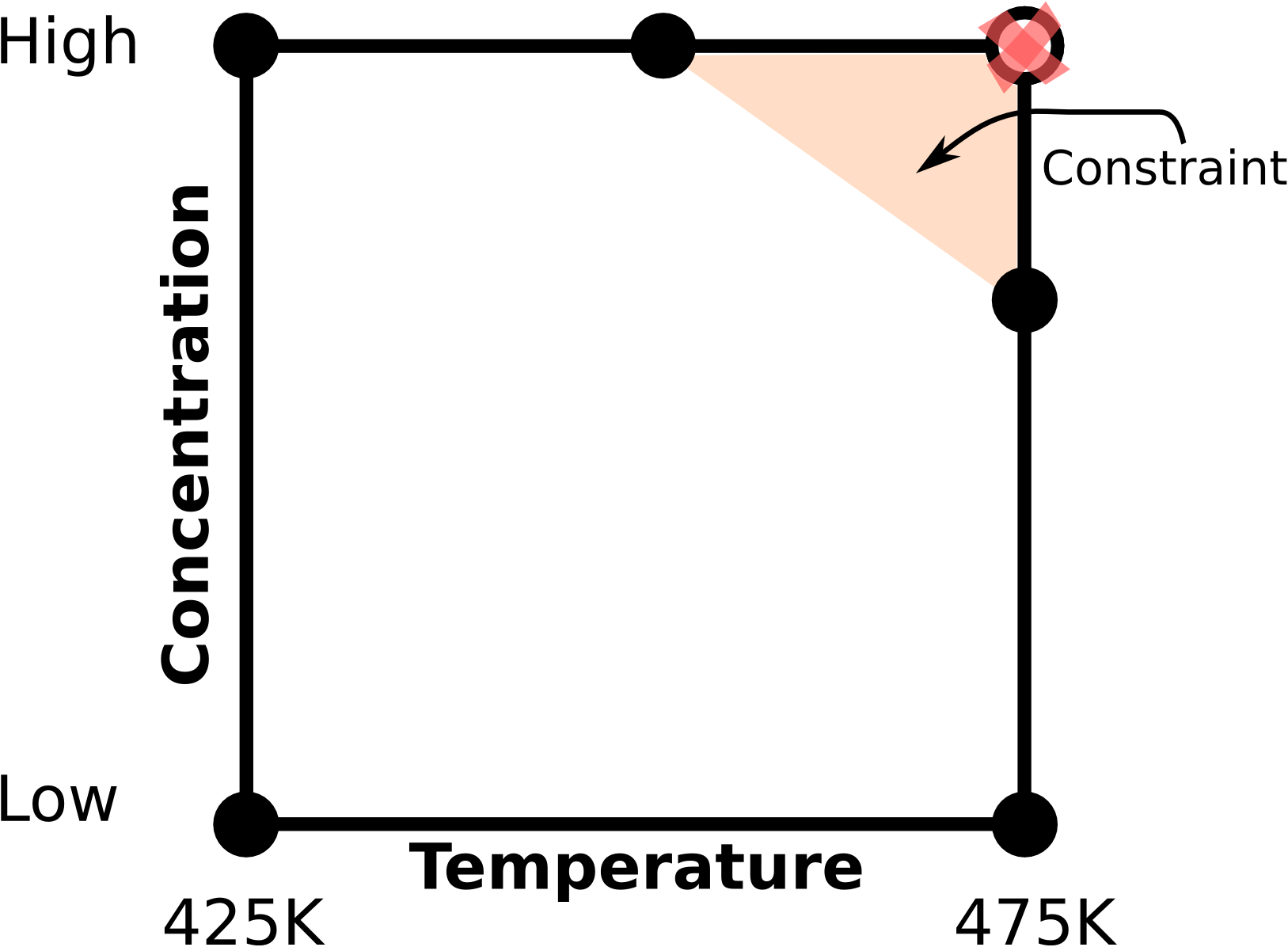
Unfortunately, these 5 runs do not form an orthogonal (independent) \(\mathbf{X}\) matrix anymore. We have lost orthogonality. We have also reduced the space (or volume when we have 3 or more factors) spanned by the factorial design.

It is easy to find experiments that obey the constraints for 2-factor cases: run them on the corner points. But for 3 or more factors the constraints form planes that cut through a cube. We then use optimal designs to determine where to place our experiments. A D-optimal design works well for constraint-handling because it finds the experimental points that would minimize the loss of orthogonality (i.e. they try to achieve the most orthogonal design possible). A compact way of stating this is to maximize the determinant of \(\mathbf{X}^T\mathbf{X}\), which is why it is called D-optimal (it maximizes the determinant).

These designs are generated by a computer, using iterative algorithms. See the D-optimal reference in the section on optimal designs for more information.

5.21.3. Mixture designs

Recipe experiments, where the factors are ingredient proportions that must sum to a constant, need their own designs and models. This topic has its own section: see mixture experiments.