
 Download PDF of entire book
4.10. More than one variable: multiple linear regression (MLR)
We now move to including more than one explanatory \(\mathrm{x}\) variable in the linear model. We will:
introduce some matrix notation for this section
show how the optimization problem is solved to estimate the model parameters
how to interpret the model coefficients
extend our tools from the previous section to analyze the MLR model
use integer (yes/no or on/off) variables in our model.
First some motivating examples:
A relationship exists between \(x_1\) = reactant concentration and \(x_2\) = temperature with respect to \(y\) = reaction rate. We already have a linear model between \(y = b_0 + b_1x_1\), but we want to improve our understanding of the system by learning about the temperature effect, \(x_2\).
We want to predict melt index in our reactor from the reactor temperature, but we know that the feed flow and pressure are also good explanatory variables for melt index. How do these additional variables improve the predictions?
We know that the quality of our plastic product is a function of the mixing time, and also the mixing tank in which the raw materials are blended. How do we incorporate the concept of a mixing tank indicator in our model?
4.10.1. Multiple linear regression: notation
To help the discussion below it is useful to omit the least squares model’s intercept term. We do this by first centering the data.
This indicates that if we fit a model where the \(\mathrm{x}\) and \(\mathrm{y}\) vectors are first mean-centered, i.e. let \(x = x_\text{original} - \text{mean}\left(x_\text{original} \right)\) and \(y = y_\text{original} - \text{mean}\left(y_\text{original} \right)\), then we still estimate the same slope for \(b_1\), but the intercept term is zero. All we gain from this is simplification of the subsequent analysis. Of course, if you need to know what \(b_0\) was, you can use the fact that \(b_0 = \overline{y} - b_1 \overline{x}\). Nothing else changes: the \(R^2, S_E, S_E(b_1)\) and all other model interpretations remain the same. You can easily prove this for yourself.
So in the rest of the this section we will omit the model’s intercept term, since it can always be recovered afterwards.
The general linear model is given by:
And writing the last equation \(n\) times over for each observation in the data:
where:
\(\mathbf{y}\): \(n \times 1\)
\(\mathbf{X}\): \(n \times k\)
\(\mathbf{b}\): \(k \times 1\)
\(\mathbf{e}\): \(n \times 1\)
4.10.2. Estimating the model parameters via optimization
As with the simple least squares model, \(y = b_0 + b_1 x\), we aim to minimize the sum of squares of the errors in vector \(\mathbf{e}\). This least squares objective function can be written compactly as:
\[\begin{split}\begin{array}{rl} f(\mathbf{b}) &= \mathbf{e}^T\mathbf{e} \\ &= \left(\mathbf{y} - \mathbf{X} \mathbf{b} \right)^T \left( \mathbf{y} - \mathbf{X} \mathbf{b} \right) \\ &= \mathbf{y}^T\mathbf{y} - 2 \mathbf{y}^T\mathbf{X}\mathbf{b} + \mathbf{b}^T\mathbf{X}^T\mathbf{X}\mathbf{b} \end{array}\end{split}\]
Taking partial derivatives with respect to the entries in \(\mathbf{b}\) and setting the result equal to a vector of zeros, you can prove to yourself that \(\mathbf{b} = \left( \mathbf{X}^T\mathbf{X} \right)^{-1}\mathbf{X}^T\mathbf{y}\). You might find the Matrix Cookbook useful in solving these equations and optimization problems.
Three important relationships are now noted:
\(\mathcal{E}\{\mathbf{b}\} = \mathbf{\beta}\), provided the postulated linear model form is correct
\(\mathcal{V}\{\mathbf{b}\} = \left( \mathbf{X}^T\mathbf{X} \right)^{-1} \sigma_\epsilon^2\), which we estimate as \(\left( \mathbf{X}^T\mathbf{X} \right)^{-1} S_E^2\)
An estimate of the standard error is given by: \(\sigma_\epsilon \approx S_E = \sqrt{\dfrac{\mathbf{e}^T\mathbf{e}}{n-k}}\), where \(k\) is the number of parameters estimated in the model and \(n\) is the number of observations. When the data have been centered, as in this section, count the intercept in \(k\) as well: the mean used for the centering was also estimated from the data, so \(k\) is the number of slope coefficients plus one.
These relationships imply that our estimates of the model parameters are unbiased (the first line), and that the variability of our parameters is related to the \(\mathbf{X}^T\mathbf{X}\) matrix and the model’s standard error, \(S_E\).
Going back to the single variable case we showed in the section where we derived confidence intervals for \(b_0\) and \(b_1\) that:
\[\mathcal{V}\{b_1\} = \dfrac{S_E^2}{\sum_j{\left( x_j - \overline{\mathrm{x}} \right)^2}}\]
Notice that the estimated matrix form, \(\left( \mathbf{X}^T\mathbf{X} \right)^{-1} S_E^2\), gives exactly the same result, remembering the \(\mathrm{x}\) variables have already been centered in the matrix form. Also recall that the variability of these estimated parameters can be reduced by (a) taking more samples, thereby increasing the denominator size, and (b) by including observations further away from the center of the model.
Example
Let \(x_1 = [1, 3, 4, 7, 9, 9]\), and \(x_2 = [9, 9, 6, 3, 1, 2]\), and \(y = [3, 5, 6, 8, 7, 10]\). By inspection, the \(x_1\) and \(x_2\) variables are negatively correlated, and the \(x_1\) and \(y\) variables are positively correlated (also positive covariance). Refer to the definition of covariance in an equation from the prior section.
After mean centering the data we have that \(x_1 = [-4.5, -2.5, -1.5 , 1.5 , 3.5, 3.5]\), and \(x_2 = [4, 4, 1, -2, -4, -3]\) and \(y = [-3.5, -1.5, -0.5, 1.5, 0.5, 3.5]\). So in matrix form:
The \(\mathbf{X}^T\mathbf{X}\) and \(\mathbf{X}^T\mathbf{y}\) matrices can then be calculated as:
Notice what these matrices imply (remembering that the vectors in the matrices have been centered). The \(\mathbf{X}^T\mathbf{X}\) matrix is a scaled version of the covariance matrix of \(\mathbf{X}\). Each diagonal term is the sum of squares of a centered variable, proportional to that variable’s variance, and always a positive number. The off-diagonal terms are symmetrical, and represent the strength of the relationship between, in this case, \(x_1\) and \(x_2\). The off-diagonal terms for two uncorrelated variables would be a number close to, or equal to zero.
The inverse of the \(\mathbf{X}^T\mathbf{X}\) matrix is particularly important - it is related to the standard error for the model parameters - as in the estimate \(\left( \mathbf{X}^T\mathbf{X} \right)^{-1} S_E^2\) of \(\mathcal{V}\{\mathbf{b}\}\).
The non-zero off-diagonal elements indicate that the variance of the \(b_1\) coefficient is related to the variance of the \(b_2\) coefficient as well. This result is true for most regression models, indicating we can’t accurately interpret each regression coefficient’s confidence interval on its own.
For the two variable case, \(y = b_1x_1 + b_2x_2\), the general relationship is that:
where \(r_{12}\) is the correlation between variable \(x_1\) and \(x_2\), so \(r^2_{12}\) is its square. What happens as the correlation between the two variables increases?
4.10.3. Interpretation of the model coefficients
Let’s take a look at the case where \(y = b_1x_1 + b_2x_2\). We can plot this on a 3D plot, with axes of \(x_1\), \(x_2\) and \(y\):
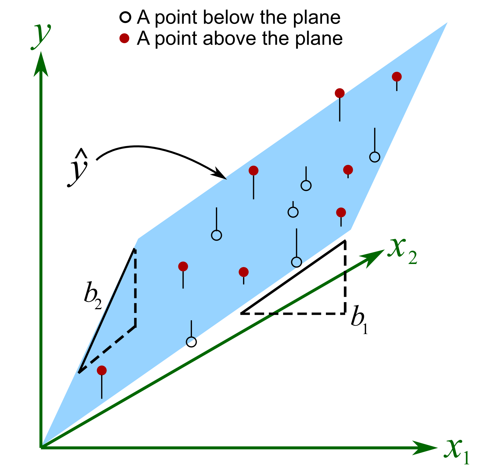
The points are used to fit the plane by minimizing the sum of square distances shown by vertical lines from each point to the plane. The interpretation of the slope coefficients for \(b_1\) and \(b_2\) is not the same as for the case with just a single \(\mathrm{x}\) variable.
When we have multiple \(\mathrm{x}\) variables, then the value of coefficient \(b_1\) is the average change we would expect in \(\mathbf{y}\) for a one unit change in \({x}_1\) provided we hold \({x}_2\) fixed. It is the last part that is new: we must assume that other \(\mathrm{x}\) variables are fixed.
For example, let \(y = b_T T + b_S S = -0.52 T + 3.2 S\), where \(T\) is reactor temperature in Kelvin, and \(S\) is substrate concentration in g/L, and \(y\) is yield in \(\mu\text{g}\), for a bioreactor reactor system. The \(b_T = -0.52 \mu\text{g}/\text{K}\) coefficient is the decrease in yield for every 1 Kelvin increase in temperature, holding the substrate concentration fixed.
This is a good point to introduce some terminology you might come across. Imagine you have a model where \({y}\) is the used vehicle price and \({x}_1\) is the mileage on the odometer (we expect that \(b_1\) will be negative) and \({x}_2\) is the number of doors on the car. You might hear the phrase: “the effect of the number of doors, controlling for mileage, is not significant”. The part “controlling for …” indicates that the controlled variable has been added to regression model, and its effect is accounted for. In other words, for two vehicles with the same mileage, the coefficient \(b_2\) indicates whether the second hand price increases or decreases as the number of doors on the car changes (e.g. a 2-door vs a 4-door car).
In the prior example, we could say: the effect of substrate concentration on yield, controlling for temperature, is to increase the yield by 3.2 \(\mu\text{g}\) for every increase in 1 g/L of substrate concentration.
4.10.3.1. Fitting an MLR model in Python
In the single-x section we built a model on the
distillation tower data using only InvTemp3 as a predictor of VapourPressure. We now
extend that model by adding a second predictor, InvPressure1 (the inverse of a pressure
measurement). The OLS class requires almost no change: we simply pass a list of column
names instead of a single one.
Python, 34 lines
import pandas as pd
from process_improve.regression import OLS

distill = pd.read_csv(
    "https://openmv.net/file/distillation-tower.csv"
)
build = distill.iloc[:150]
test = distill.iloc[150:]

# Specifying the predictors as a list lets us
# add or remove variables without touching
# the rest of the code:
predictors = ["InvTemp3", "InvPressure1"]

X_build_MLR = build[predictors].values
y_build = build["VapourPressure"].values

full_model = OLS()
full_model.fit(X=X_build_MLR, y=y_build)

# Residuals on the building data:
predict_MLR_build = full_model.predict(X_build_MLR)
errors_MLR_build = y_build - predict_MLR_build
avg_absolute_error_MLR_build = (
    pd.Series(errors_MLR_build).abs().mean()
)
print(
    f"MLR building-data average absolute error "
    f"= {avg_absolute_error_MLR_build:.3f}"
)

pd.Series(errors_MLR_build).plot(
    title="MLR residuals (Actual - Predicted)",
)
The same model is then assessed on the held-out test partition. Compare the average absolute error and standard deviation against the values reported in the single-predictor case: a useful additional predictor should reduce both numbers, and leave the residual time series free of obvious drift or structure.
Python, 16 lines
X_test_MLR = test[predictors].values
y_test = test["VapourPressure"].values

predict_MLR_test = full_model.predict(X_test_MLR)
errors_MLR_test = y_test - predict_MLR_test

avg_absolute_error_MLR_test = (
    pd.Series(errors_MLR_test).abs().mean()
)
std_error_MLR_test = errors_MLR_test.std()

print(
    f"MLR testing-data average absolute error "
    f"= {avg_absolute_error_MLR_test:.3f}, "
    f"std. dev. = {std_error_MLR_test:.3f}"
)
4.10.4. \(R^2\) never decreases as terms are added
The discussion of \(R^2\) in the model analysis section cautioned that \(R^2\) can be increased simply by adding terms to the model. On the building data, \(R^2\) cannot decrease when a term is added: the optimization is free to set the new coefficient to zero and keep the previous fit, so the fit can only stay the same or improve. On the distillation data the second predictor is a useful one:
Python, 10 lines
import numpy as np

# `build`, `y_build`, `X_build_MLR` and `full_model`
# are from the code sections earlier in this chapter.
X_one = build[["InvTemp3"]].values
r2_one = OLS().fit(X_one, y_build).score(X_one, y_build)
r2_two = full_model.score(X_build_MLR, y_build)

# R-squared: 0.781, then 0.938
print(f"{r2_one:.3f}  {r2_two:.3f}")
Adding InvPressure1 raises \(R^2\) from 0.781 to 0.938 and also improves the testing-data
error: that predictor carries real information. A useless term also raises \(R^2\). To see
by how much, append one column of random noise to the two real predictors as a third “predictor”
and refit:
Python, 8 lines
noise_col = np.random.default_rng(0).normal(
    size=(len(X_build_MLR), 1)
)
X_noise = np.hstack([X_build_MLR, noise_col])
r2_noise = OLS().fit(X_noise, y_build).score(X_noise, y_build)

print(f"{r2_two:.5f}  {r2_noise:.5f}")
# 0.93831  0.93847
On these 150 building rows the noise column raises \(R^2\) from 0.93831 to 0.93847; the size of the increase varies with the random seed, and its expected value for a column that carries no information is \((1 - R^2)/(n - k) = (1 - 0.93831)/(150 - 3) = 0.00042\), where \(n\) is the number of observations and \(k\) is the number of parameters (intercept included) already in the model. With many observations, one junk column can only absorb a small share of the variance. The fewer the observations relative to the number of parameters, the larger the share a useless term can absorb. The 14 runs of the bioreactor yields data set (used again in the exercises) make the effect plainly visible:
Python, 27 lines
bio = pd.read_csv(
    "https://openmv.net/file/bioreactor-yields.csv"
)
# Code the Yes/No baffles column as 1/0:
bio["baffles"] = (bio["baffles"] == "Yes").astype(int)
y_bio = bio["yield"].values
n_bio = len(bio)  # only 14 runs
X_real = bio[["temperature", "speed", "baffles"]].values

rng = np.random.default_rng(39)
noise = rng.normal(size=(n_bio, 10))

# Fit the model with 0, 1, 2 and 3 columns of pure
# random noise appended as extra "predictors":
for extra in range(0, 4):
    X_bio = np.hstack([X_real, noise[:, :extra]])
    model = OLS().fit(X_bio, y_bio)
    r2 = model.score(X_bio, y_bio)
    k = X_bio.shape[1] + 1  # parameters, incl. intercept
    r2_adj = 1 - (1 - r2) * (n_bio - 1) / (n_bio - k)
    print(f"{extra} noise columns: R2 = {r2:.3f}, "
          f"adjusted R2 = {r2_adj:.3f}")

# 0 noise columns: R2 = 0.866, adjusted R2 = 0.826
# 1 noise columns: R2 = 0.875, adjusted R2 = 0.819
# 2 noise columns: R2 = 0.885, adjusted R2 = 0.813
# 3 noise columns: R2 = 0.894, adjusted R2 = 0.802
Each noise column raises \(R^2\) by roughly 0.01, from 0.866 with the three real predictors to 0.894 with three junk columns added, even though the junk columns carry no information about the yield. Kept up, this reaches \(R^2 = 1.0\) exactly when the parameter count reaches the number of runs: with all 10 noise columns, 3 real predictors and the intercept, 14 parameters fit the 14 runs perfectly. The adjusted \(R^2\), which divides each sum of squares by its degrees of freedom, moves in the opposite direction, falling from 0.826 to 0.802: the penalty for each extra term outweighs its accidental gain in fit. This is why \(R^2\) on the building data cannot tell you whether a new term earns its place in the model. Two better checks were introduced earlier: the adjusted \(R^2\), and the prediction error on testing data, which a noise column will generally make worse.
4.10.5. Integer (dummy, indicator) variables in the model
Now that we have introduced multiple linear regression to expand our models, we also consider these sort of cases:
We want to predict yield, but want to indicate whether a radial or axial impeller was used in the reactor and learn whether it has any effect on yield.
Is there an important difference when we add the catalyst first and then the reactants, or the reactants followed by the catalyst?
Use an indicator variable to show if the raw material came from the supplier in Spain, India, or Vietnam and interpret the effect of supplier on yield.
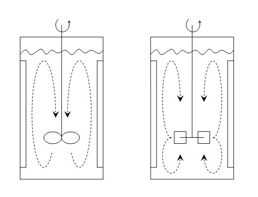
Axial and radial blades; figure from Wikipedia
We will start with the simplest case, using the example of the radial or axial impeller. We wish to understand the effect on yield, \(y [\mu\text{g}]\), as a function of the impeller type, and impeller speed, \(x\).
where \(d_i = 0\) if an axial impeller was used, or \(d_i = 1\) if a radial impeller was used. All other least squares assumptions hold, particularly that the variance of \(y_i\) is unrelated to the value of \(d_i\). For the initial discussion let’s assume that \(\beta_1 = 0\), then geometrically, what is happening here is:
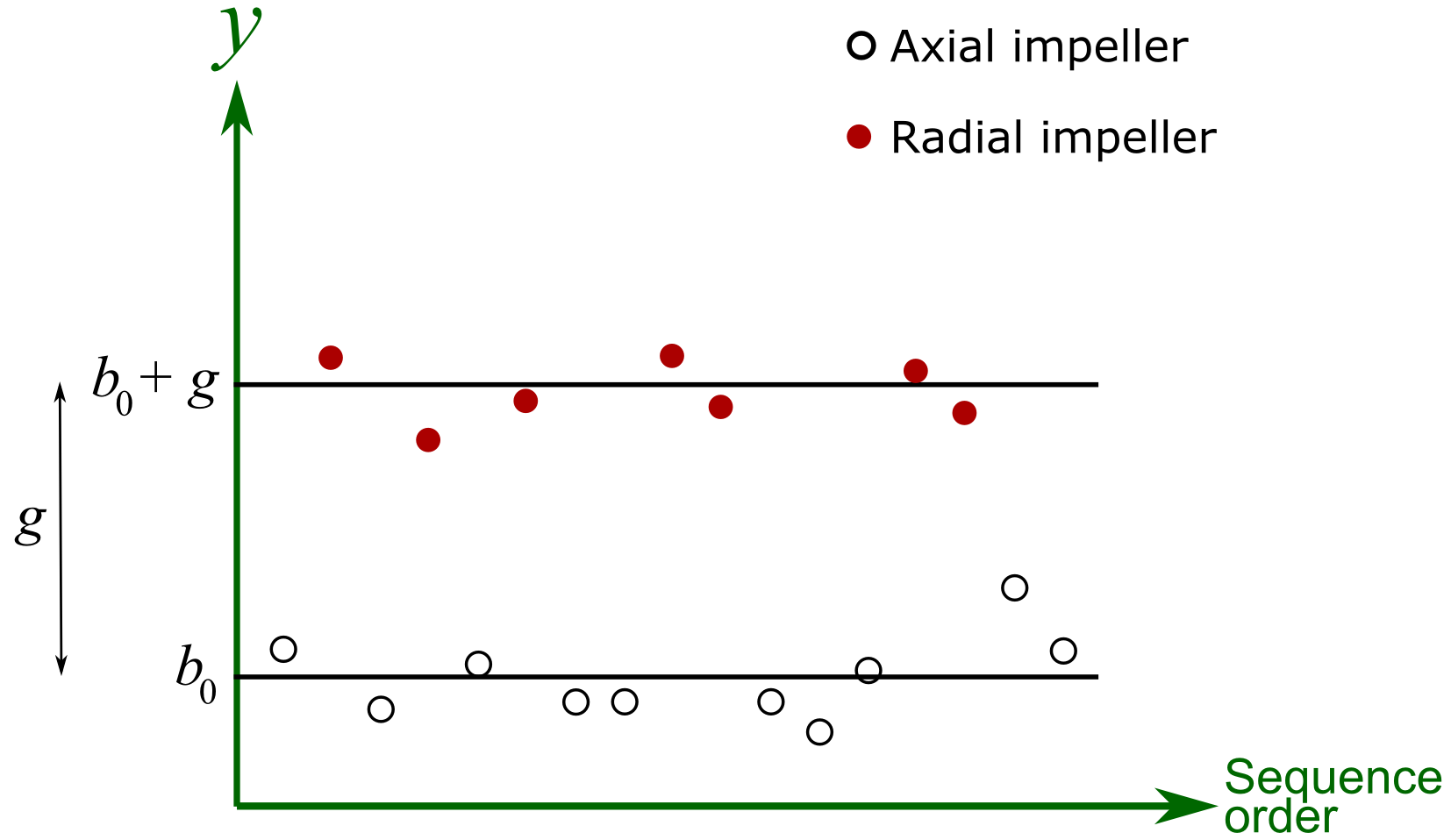
The \(\gamma\) parameter, estimated by \(g\), is the difference in intercept when using a different impeller type. Note that the lines are parallel.
Now if \(\beta_1 \neq 0\), then the horizontal lines in the above figure are tilted, but still parallel to each other. Nothing else is new here, other than the representation of the variable used for \(d_i\). The interpretation of its coefficient, \(g\), is the same as with any other least squares coefficient. In this particular example, had \(g = -56 \mu\text{g}\), it would indicate that the average decrease in yield is 56 \(\mu\text{g}\) when using a radial impeller.
The rest of the analysis tools for least squares models can be used quite powerfully. For example, a 95% confidence interval for the impeller variable might have been:
which would indicate the impeller type has no significant effect on the yield amount, the \(y\)-variable.
Integer variables are also called dummy variables or indicator variables. Really what is happening here is the same concept as for multiple linear regression, the equation of a plane is being estimated. We only use the equation of the plane at integer values of \(d\), but mathematically the underlying plane is actually continuous.
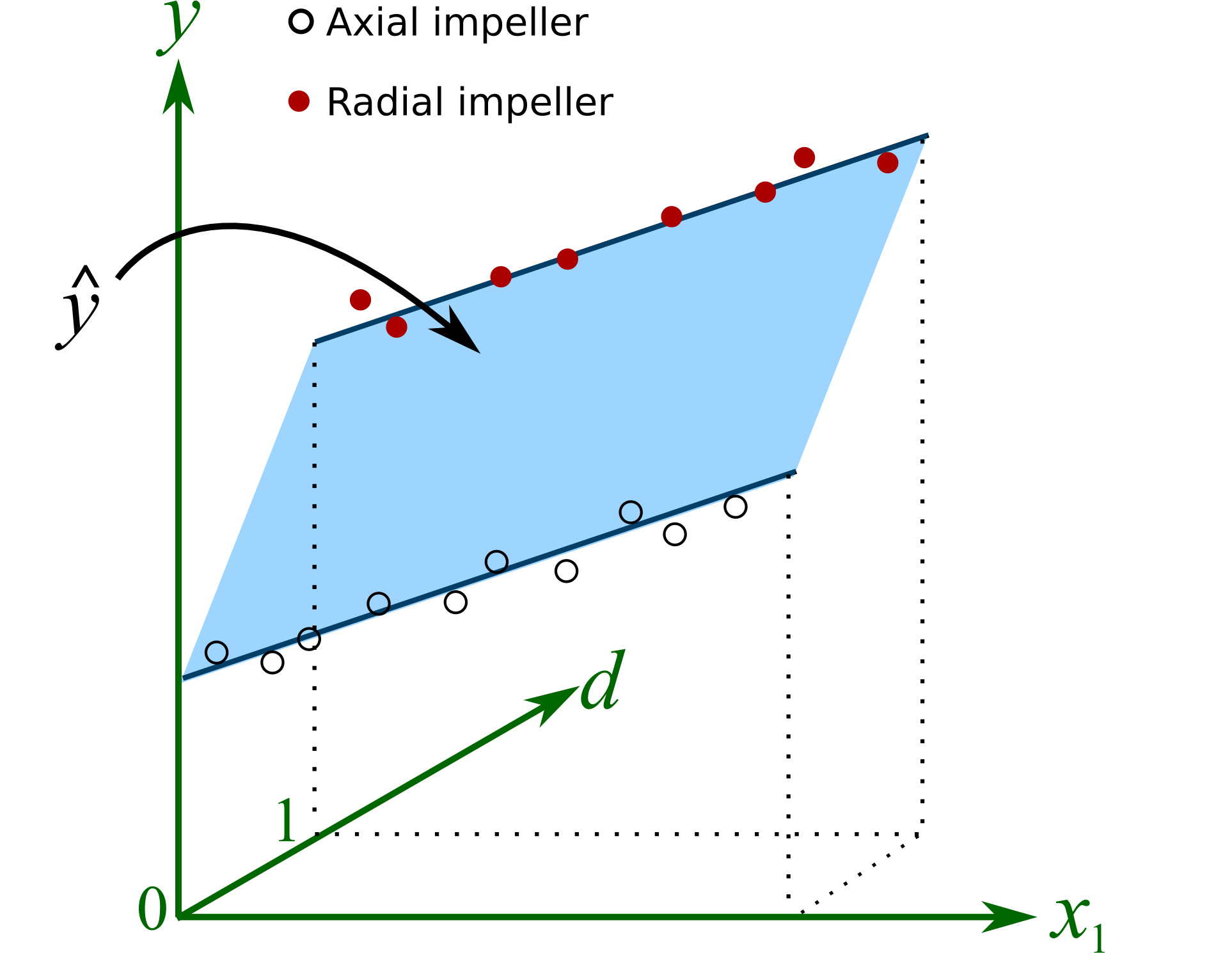
We have to introduce additional terms into the model if we have integer variables with more than 2 levels. In general, if there are \(p\)-levels, then we must include \(p-1\) terms. For example, if we wish to test the effect of \(y\) = yield achieved from the raw material supplier in Spain, India, or Vietnam, we could code:
Spain: \(d_{i1} = 0\) and \(d_{i2} = 0\)
India: \(d_{i1} = 1\) and \(d_{i2} = 0\)
Vietnam: \(d_{i1} = 0\) and \(d_{i2} = 1\).
and solve for the least squares model: \(y = \beta_0 + \beta_1x_1 + \ldots + \beta_k x_k + \gamma_1 d_1 + \gamma_2 d_2 + \varepsilon\), where \(\gamma_1\) is the effect of the Indian supplier, holding all other terms constant (i.e. it is the incremental effect of India relative to Spain); \(\gamma_2\) is the incremental effect of the Vietnamese supplier relative to the base case of the Spanish supplier. Because of this somewhat confusing interpretation of the coefficients, sometimes people will assume they can sacrifice an extra degree of freedom, but introduce \(p\) new terms for the \(p\) levels of the integer variable, instead of \(p-1\) terms.
Spain: \(d_{i1} = 1\) and \(d_{i2} = 0\) and \(d_{i3} = 0\)
India: \(d_{i1} = 0\) and \(d_{i2} = 1\) and \(d_{i3} = 0\)
Vietnam: \(d_{i1} = 0\) and \(d_{i2} = 0\) and \(d_{i3} = 1\)
and \(y = \beta_0 + \beta_1x_1 + \ldots + \beta_k x_k + \gamma_1 d_1 + \gamma_2 d_2 + \gamma_3 d_3 + \varepsilon\), where the coefficients \(\gamma_1, \gamma_2\) and \(\gamma_3\) are assumed to be more easily interpreted. However, calculating this model will fail, because there is a built-in perfect linear combination. The \(\mathbf{X}^T\mathbf{X}\) matrix is not invertible.