5.9.8. Saturated designs for screening

A saturated design is one in which the number of runs equals the number of parameters being estimated, so there are no degrees of freedom left over. The model fits the data exactly, every residual is zero, and no classical standard error can be computed. A saturated design can be likened to a well trained doctor asking you a few, but very specific, questions to identify a disease or problem. On the other hand, if you just sit there and tell the doctor all your symptoms, you may or may not get an accurate diagnosis. Designed experiments, like visiting this doctor, shorten the time required to identify the major effects in a system, and to do so as accurately as possible, within a limited budget.

Saturated designs are most suited for screening, and are a natural choice when you are investigating a new system with many factors. These designs are usually of resolution III and estimate all the main effects with a low number of experiments. A \(2^{7-4}_{\text{III}}\) factorial, for instance, spends its 8 runs on an intercept and 7 main effects, so it is saturated.

For example, a \(2^{7-4}_{\text{III}}\) factorial, introduced in the section on highly fractionated designs, will screen 7 factors in 8 experiments. Once you have run the 8 experiments you can quickly tell which subset of the 7 factors are actually important, and spend the rest of your budget on clearly understanding these effects and their interactions. Bear in mind that there is a risk of confounding, as previously described in that section.

Let’s see how by continuing the previous example, repeated again below with the corresponding values of \(y\). Recall it was a set of eight experiments in seven factors:

Experiment	A	B	C	D=AB	E=AC	F=BC	G=ABC	\(y\)
1	\(-\)	\(-\)	\(-\)	\(+\)	\(+\)	\(+\)	\(-\)	77.1
2	\(+\)	\(-\)	\(-\)	\(-\)	\(-\)	\(+\)	\(+\)	68.9
3	\(-\)	\(+\)	\(-\)	\(-\)	\(+\)	\(-\)	\(+\)	75.5
4	\(+\)	\(+\)	\(-\)	\(+\)	\(-\)	\(-\)	\(-\)	72.5
5	\(-\)	\(-\)	\(+\)	\(+\)	\(-\)	\(-\)	\(+\)	67.9
6	\(+\)	\(-\)	\(+\)	\(-\)	\(+\)	\(-\)	\(-\)	68.5
7	\(-\)	\(+\)	\(+\)	\(-\)	\(-\)	\(+\)	\(-\)	71.5
8	\(+\)	\(+\)	\(+\)	\(+\)	\(+\)	\(+\)	\(+\)	63.7

Use a least squares model to estimate the coefficients in the model:

\[\begin{split}\mathbf{y} &= \mathbf{Xb} \\ \mathbf{b} &= \left(\mathbf{X}^T\mathbf{X}\right)^{-1}\mathbf{X}^T\mathbf{y}\end{split}\]

where \(\mathbf{b} = [b_0, b_A, b_B, b_C, b_D, b_E, b_F, b_G]\). The matrix \(\mathbf{X}\) is essentially a copy of the above table, but with an added column of 1’s for the intercept term. Notice that the \(\mathbf{X}^T\mathbf{X}\) matrix will be diagonal. Make sure you can calculate \(\mathbf{X}^T\mathbf{X}\) by hand, at least once. It is also straightforward to calculate the solution vector (by hand!), which you can confirm to be \(\mathbf{b} = [70.7, -2.3, 0.1, -2.8, -0.4, 0.5, -0.4, -1.7]\).

How do you assess which main effects are important? There are eight data points and eight parameters, so there are no degrees of freedom and the residuals are all zero. In this case you have to use a Pareto plot, which requires that your variables have been suitably scaled in order to judge importance of the main effects relative to each other. The Pareto plot would be given as shown below, and as usual, it does not show the intercept term.

Python, 57 lines

import itertools
import numpy as np
import pandas as pd
import statsmodels.api as sm

pd.options.plotting.backend = "plotly"

# Create vectors for each factor in the experiment.
# itertools.product varies the last column fastest, so we label
# the columns C, B, A to obtain standard (Yates) order, where
# factor A alternates fastest. This matches the run table above.
design = pd.DataFrame(
    list(itertools.product([-1, +1],
                           [-1, +1],
                           [-1, +1])),
    columns=["C", "B", "A"],
)[["A", "B", "C"]]
A = design["A"].to_numpy()
B = design["B"].to_numpy()
C = design["C"].to_numpy()
D = A * B
E = A * C
F = B * C
G = A * B * C
y = np.array([77.1, 68.9, 75.5, 72.5,
              67.9, 68.5, 71.5, 63.7])

X = np.column_stack([A, B, C, D, E, F, G])
X = sm.add_constant(X)
demo = sm.OLS(y, X).fit()
print(demo.summary())

# OK, now we are ready to generate the Pareto plot.
# Sort the absolute coefficient values, dropping
# the intercept (matching the R paretoPlot conventions).
names = ["A", "B", "C", "D", "E", "F", "G"]
effects = pd.Series(
    np.abs(demo.params[1:]),
    index=names,
).sort_values()
fig = effects.plot.bar(orientation="h")
fig.update_layout(
    xaxis_title_text="|effect|",
    yaxis_title_text="Factor",
    showlegend=False,
)
fig.show()

# Try getting the results manually:
XtX = X.T @ X
print("The XtX matrix is:")
print(XtX)

Xty = X.T @ y
b = np.linalg.solve(XtX, Xty)
print("The solution vector is:")
print(b)

R, 39 lines

# Create vectors for each factor in the experiment
A = B = C = c(-1, +1)
design = expand.grid(A=A, B=B, C=C)
A = design$A
B = design$B
C = design$C
D = A*B
E = A*C
F = B*C
G = A*B*C
y = c(77.1, 68.9, 75.5, 72.5, 67.9, 68.5, 71.5, 63.7)

demo = lm(y ~ A + B + C + D + E + F + G)
summary(demo)

# OK, now we are ready to generate the Pareto plot.
# Let's use a library to do that for us.

# library(pid) <-- best to use this!
# It is better to uncomment and use the line above.

# But this embedded R script on this website does not have the
# "pid" library available. So we will load the required function
# from an external server instead:
source('https://yint.org/paretoPlot.R')

# And now we can generate the plot:
paretoPlot(demo)

# Try getting the results manually:
X_matrix = model.matrix(demo)
XtX <- t(X_matrix) %*% X_matrix
print('The XtX matrix is:')
print(XtX)

Xty <- t(X_matrix) %*% y
b = solve(XtX) %*% Xty
print('The solution vector is:')
print(b)

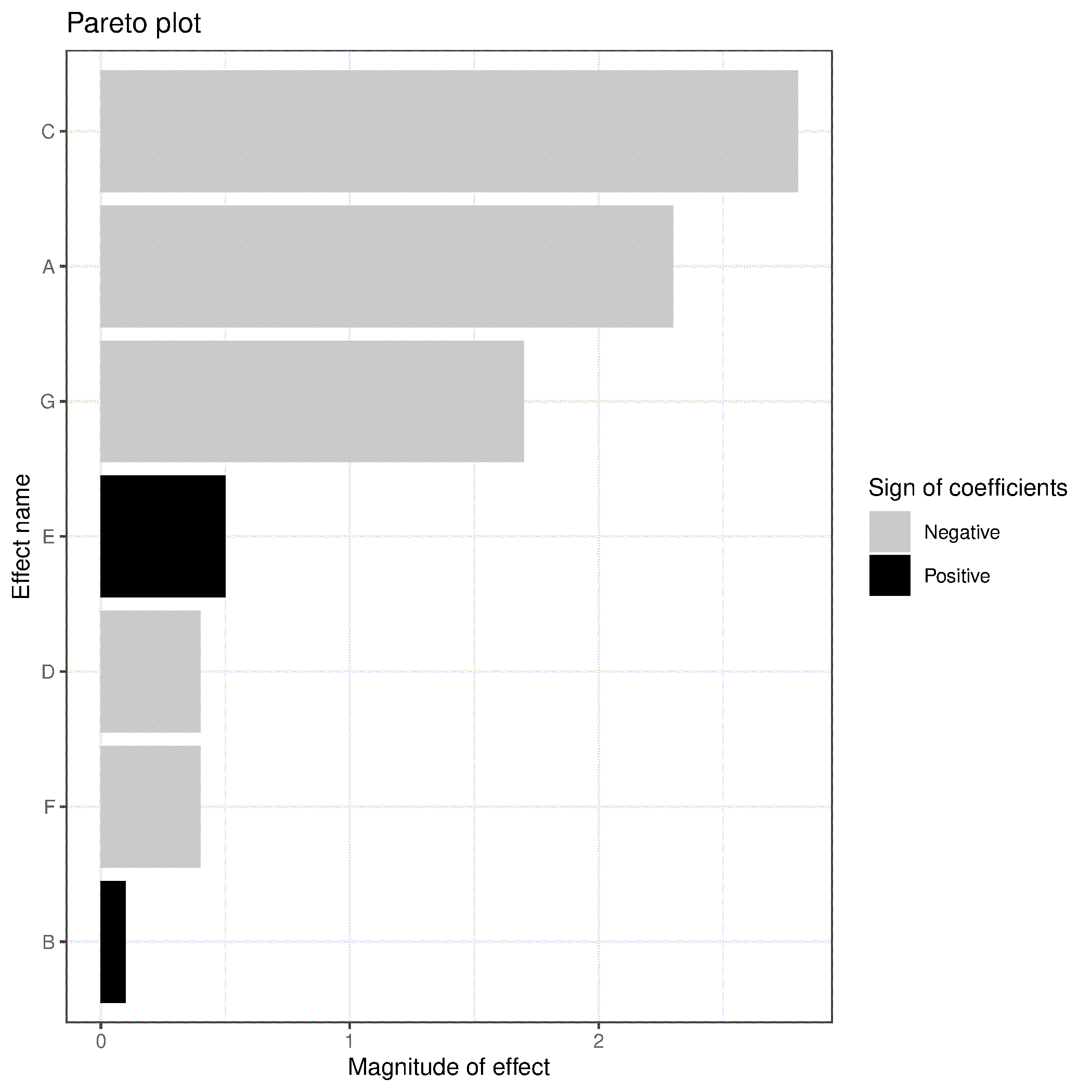
The Pareto plot ranks the effects; to place an objective cutoff on this zero-degrees-of-freedom design we apply Lenth’s method to the seven coefficients:

Python, 10 lines

from scipy import stats

coeffs = b[1:]                       # the seven effect coefficients, A ... G
abs_c = np.abs(coeffs)
s0 = 1.5 * np.median(abs_c)
pse = 1.5 * np.median(abs_c[abs_c < 2.5 * s0])
ME = stats.t.ppf(0.975, len(coeffs) / 3) * pse
print(f"PSE = {pse:.2f}, ME = {ME:.2f}")     # PSE = 0.60, ME = 2.26
for name, c in zip(names, coeffs):
    print(name, round(c, 2), abs(c) > ME)

In the Pareto plot, each bar is coloured by the sign of its effect (orange for a positive coefficient, blue for a negative one), and the dashed vertical line is the Lenth margin of error. Here both of the largest effects, A and C, are negative, so they appear in blue but still extend past the margin-of-error line.

The pseudo standard error is \(\text{PSE} = 0.60\), giving a margin of error of \(\text{ME} = 2.26\). Two effects clear it: A (\(|c| = 2.3\)) and C (\(|c| = 2.8\)). The next largest, G (\(|c| = 1.7\)), falls just below the margin, so on this evidence it is a candidate rather than a confirmed effect: a follow-up experiment would be needed to settle it. Recall too that each estimate is confounded: for the main effect E, for example, \(\widehat{\beta}_{\mathbf{E}} \rightarrow\) E + AC + BG + DF, so even a clearly significant reading could arise from the main effect or from any of its aliases.

The factors B, D and F are small and can be set aside in this region. Future experiments should focus on A and C, on confirming G, and on resolving the aliasing among their interactions. We show how to reuse these existing 8 experiments, adding a few new ones, in the next section on design foldover and by understanding projectivity.

A side note on screening designs is a mention of Plackett and Burman designs. These designs can sometimes be of greater use than a highly fractionated design. A fractional factorial must have \(2^{k-p}\) runs, for integers \(k\) and \(p\): i.e. either \(4, 8, 16, 32, 64, 128, \ldots\) runs. Plackett-Burman designs are screening designs that can be run in any multiple of 4, i.e. \(12, 16, 20, 24, \ldots\) runs. The non-geometric cases (12, 20, 24, 28, …), which are not powers of 2, are the ones that a fractional factorial cannot provide. The Box, Hunter, and Hunter book has more information in Chapter 7, but another interesting paper on these topic is by Box and Bisgaard: “What can you find out from 12 experimental runs?”, which shows how to screen for 11 factors in 12 experiments.

5.9.8.1. Three principles behind screening: sparsity, hierarchy, and heredity

Screening works because real systems tend to behave in a particular way. Three empirical principles describe that behaviour. Together they explain why a saturated design can find the important factors, and how to build a model from the results. All three are discussed at length in Goos and Jones.

Sparsity. The principle of effect sparsity states that only a few of the many factors studied drive most of the variation in the response. This is the experimental form of the Pareto principle: a small number of causes account for a large part of the effect. The saturated \(2^{7-4}_{\text{III}}\) design above relied on it. It spent 8 runs on 7 factors and found that only A, C, and G mattered. Sparsity is what lets the Pareto plot separate the few large effects from the many small ones. As the number of active effects grows towards half the number of runs, that separation becomes harder to make.

Hierarchy. The principle of effect hierarchy states that main effects tend to be larger than two-factor interactions, which in turn tend to be larger than three-factor and higher-order interactions. This is why a resolution III design confounds main effects with two-factor interactions rather than confounding main effects with each other: the terms it gives up to save runs are the ones expected to be small. In model building, hierarchy suggests adding the main effects before any interaction or quadratic term.

Heredity. The principle of effect heredity concerns which interactions are plausible. Under strong heredity, a two-factor interaction \(x_i x_j\) is included in a model only if both of its parent main effects, \(x_i\) and \(x_j\), are also in the model. Under weak heredity, only one of the two parents needs to be present. Heredity is the usual reason for keeping a main effect in a model even when its own coefficient looks small: if its interaction is active, the main effect stays.

A small example shows why. Suppose the true response is \(y = 10 + 4 x_A - 2 x_B + 23 x_A x_B\), and a full factorial is run at the \(\pm 1\) levels. A model that keeps only the intercept and the interaction, dropping both main effects, fits the four corner points with \(y = 10 + 23 x_A x_B\). Its coefficients are close to the true ones, and at most corners it predicts well. But at the corner \(x_A = +1, x_B = -1\), where the main effects and the interaction push in opposite directions, it predicts \(10 + 23(+1)(-1) = -13\), while the true value is \(10 + 4(+1) - 2(-1) + 23(+1)(-1) = -7\). Retaining the parent main effects avoids this error. A model built under strong heredity has a further technical advantage: its predictions do not change if the factors are rescaled.

These are tendencies, not laws. An empirical review of 113 published factorial experiments, summarised in Goos and Jones, found that hierarchy and heredity usually hold, while also noting that violations occur more often than the screening literature suggests. The same review found that most active two-factor interactions are synergistic: they reinforce the direction of their parent main effects. When the goal is to increase the response, exploiting the large main effects tends to carry the interactions along in the same direction. When the goal is to decrease it, the interactions can work against the main effects.

An important mention to readers interested in other, arguable better screening strategies, is to consider definitive screening designs.