There are five main areas where engineers use large quantities of data.
Improved process understanding
This is an implicit goal in any data analysis: either we confirm what we know about the process, or we see something unusual show up and learn from it. Plots that show, in one go, how a complex set of variables interact and relate to each other are required for this step.
Troubleshooting process problems
Troubleshooting occurs after a problem has occurred. There are many potential sources that could have caused the problem. Screening tools are required that will help isolate the variables most related to the problem. These variables, combined with our engineering knowledge, are then used to troubleshoot why the problem occurred.
Improving, optimizing and controlling processes
We have already introduced the concept of designed experiments and response surface methods. These are excellent tools to intentionally manipulate your process so that you can find a more optimal operating point, or even develop a new product. We will show how latent variable tools can be used on a large historical data set to improve process operation, and to move to a new operating point. There are also tools for applying process control in the latent variable space.
Predictive modelling (inferential sensors)
The section on least squares modelling provided you with a tool for making predictions. We will show some powerful examples of how a “difficult-to-measure” variable can be predicted in real-time, using other easy-to-obtain process data. Least squares modelling is a good tool, but it lacks some of the advantages that latent variable methods provide, such as the ability to handle highly collinear data, and data with missing values.
Process monitoring
Once a process is running, we require monitoring tools to ensure that it maintains and stays at optimal performance. We have already considered process monitoring charts for univariate process monitoring. In this section we extend that concept to monitoring multiple variables.
When industrial manufacturing and chemical engineering started to develop around the 1920’s to 1950’s, data collected from a process were, at most, just a handful of columns. These data were collected manually and often at considerable expense.
We will represent any data set as a matrix, called , where each row in contains values taken from an object of some sort. These rows, or observations could be a collection of measurements at a particular point in time, various properties on a sample of final product, or a sample of raw material from a supplier. The columns in are the values recorded for each observation. We call these the variables and there are of them.
These data sets from the 1950’s frequently had many more rows than columns, because it was expensive and time-consuming to measure additional columns. The choice of which columns to measure was carefully thought out, so that they didn’t unnecessarily duplicate the same measurement. As a result:
the columns of X were often independent, with little or no overlapping information
the variables were measured in a controlled environment, with a low amount of error
These data sets meet all the assumptions required to use the so-called “classical” tools, especially least squares modelling. Data sets that engineers currently deal with though can be of any configuration with both large and small and large and small , but more likely we have many columns for each observation.
Small N and small K
These cases are mostly for when we have expensive measurements, and they are hard to obtain frequently. Classical methods to visualize and analyze these data always work well: scatterplots, linear regression, etc.
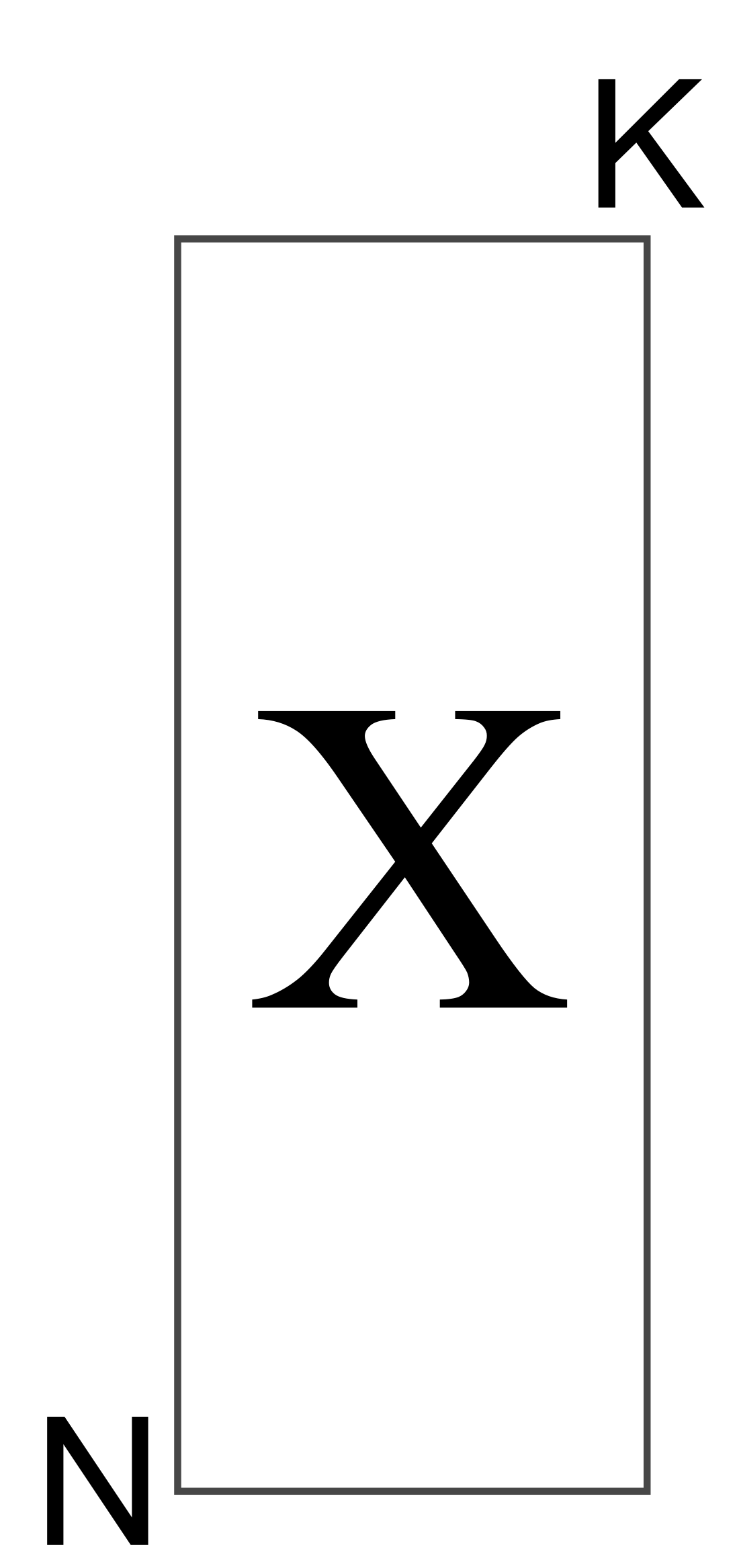
Small N and large K
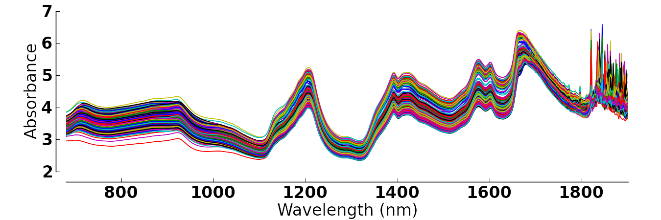
This case is common for laboratory instrumentation, particularly spectroscopic devices. In recent years we are routinely collecting large quantities of data. A typical example is with near-infrared probes embedded at-line. These probes record a spectral response at around 1000 to 2000 different wavelengths. The data are represented in using one wavelength per column and each sample appears in a row. The illustration here shows data from samples, with data recorded every 2 nm ().
Obviously not all the columns in this matrix are important; some regions are more useful than others, and columns immediately adjacent to each other are extremely similar (non-independent).
An ordinary least squares regression model, where we would like to predict some -variable from these spectral data, cannot be calculated when , since we are then estimating more unknowns than we have observations for. A common strategy used to deal with non-independence is to select only a few columns (wavelengths in the spectral example) so that . The choice of columns is subjective, so a better approach is required, such as projection to latent structures.
Large N and small K
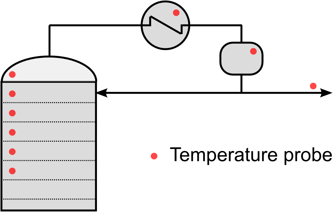
A current-day chemical refinery easily records about 2 observations (rows) per second on around 2000 to 5000 variables (called tags); generating in the region of 50 to 100 Mb of data per second.
For example, a modest size distillation column would have about 35 temperature measurements, 5 to 10 flow rates, 10 or so pressure measurements, and then about 5 more measurements derived from these recorded values.
The case of squarish matrices mostly occurs by chance: we just happen to have roughly the same number of variables as observations.
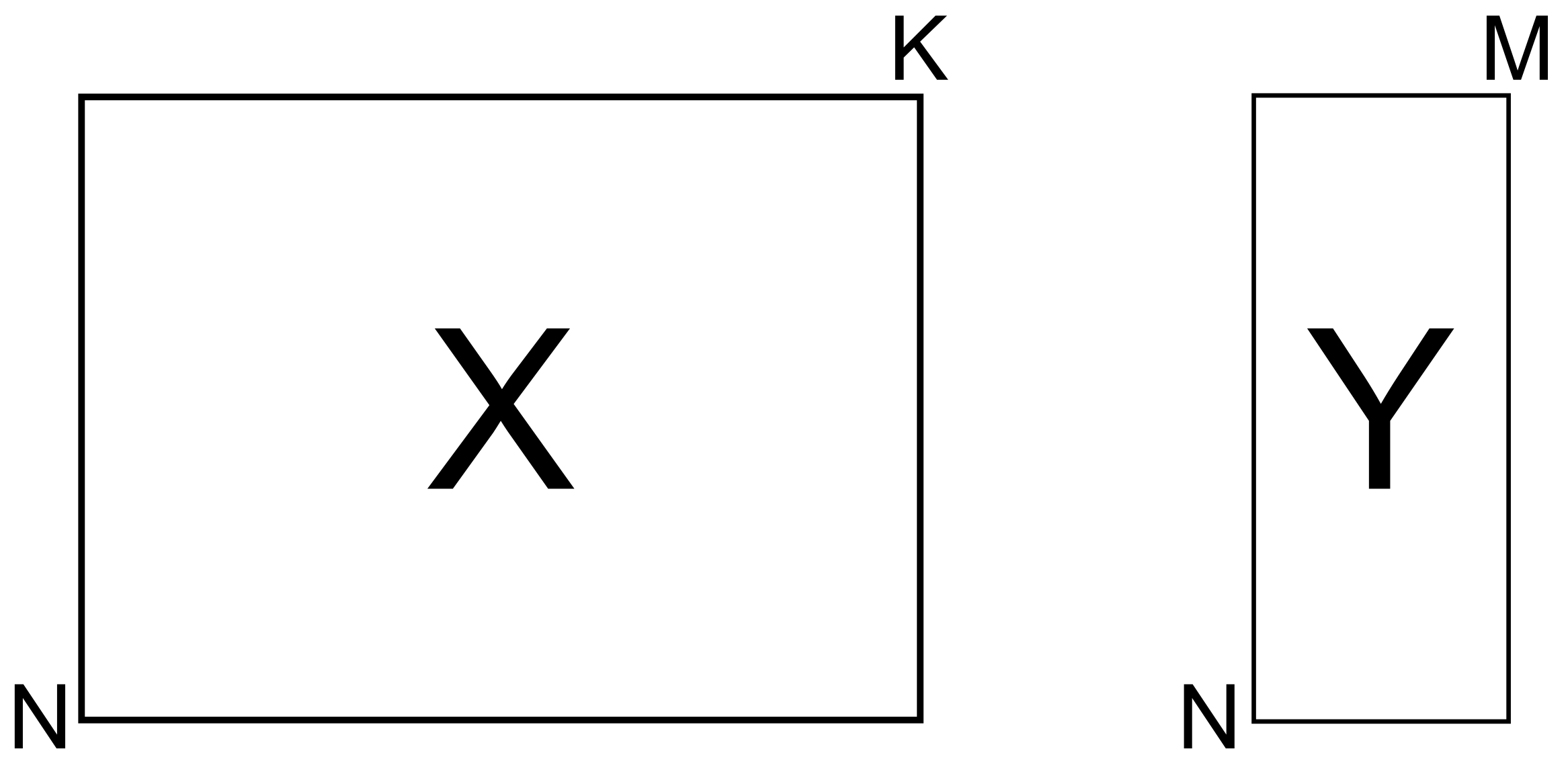
X and Y matrices
This situation arises when we would like to predict one or more variables from another group of variables. We have already seen this data structure in the least squares section where , but more generally we would like to predict several -values from the same data in .
The “classical” solution to this problem is to build and maintain different least squares models. We will see in the section on projection to latent structures that we can build a single regression model. The sections on principal component regression also investigates the above data structure, but for single -variables.
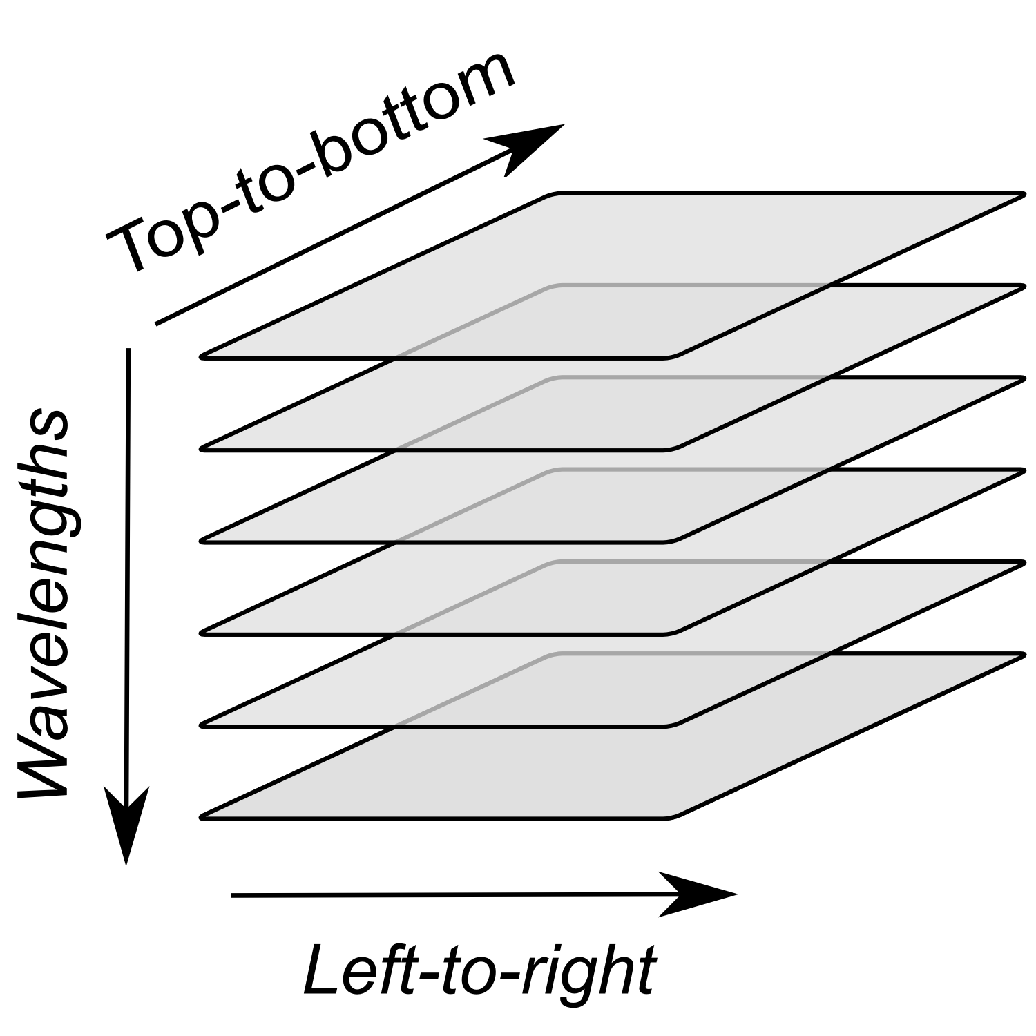
3D data sets and higher dimensions
These data tables are becoming very common, especially since 2000 onwards. A typical example is for image data from digital cameras. In this illustration a single image is taken at a point in time. The camera records the response at 6 different wavelengths, and the spatial directions (top-to-bottom and left-to-right). These values are recorded in a 3D data cube.
A fourth dimension can be added to this data if we start recording images over time. Such systems generate between 1 and 5 Mb of data per second. As with the spectral data set mentioned earlier, these camera systems generate large quantities of redundant data, because neighbouring pixels, both in time and spatially, are so similar. It is a case of high noise and little real information.
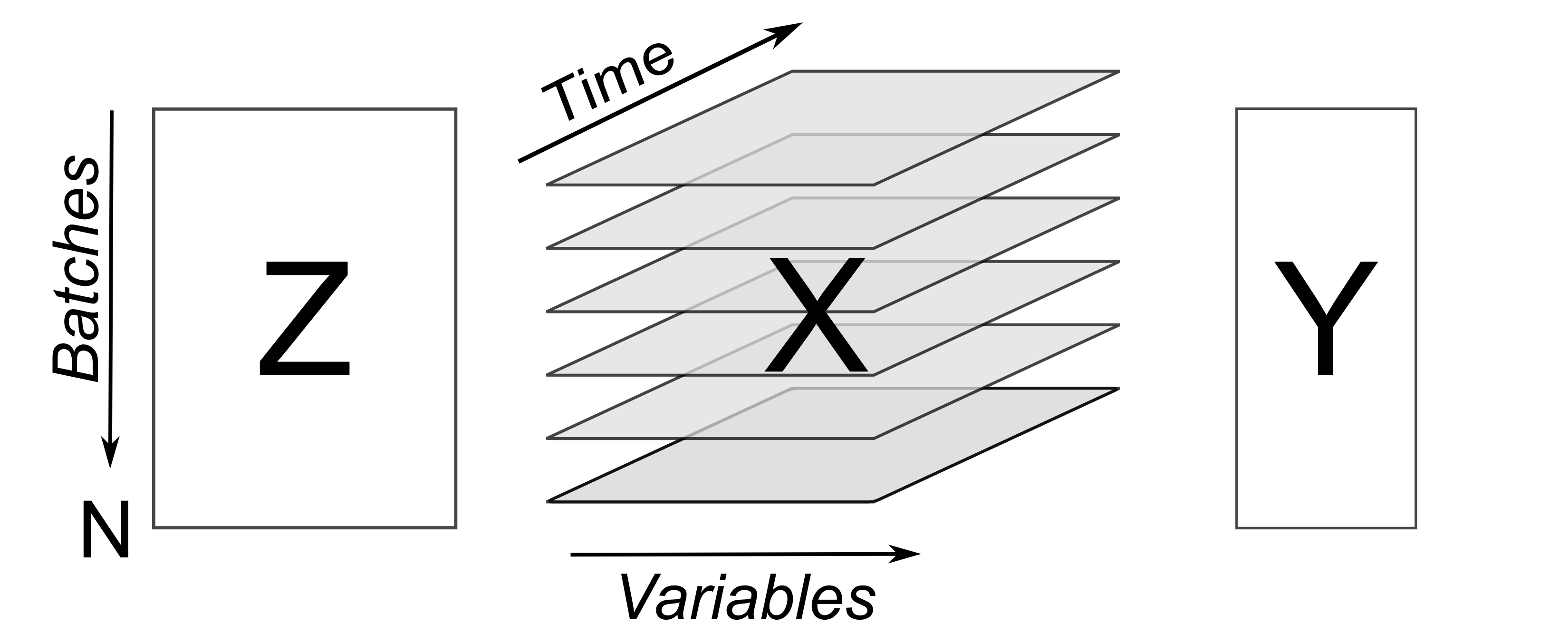
Batch data sets
Batch systems are common with high-value products: pharmaceuticals, fine-chemicals, and polymers. The matrix below contains data that describes how the batch is prepared and also contains data that is constant over the duration of the whole batch. The matrix contains the recorded values for each variable over the duration of the batch. For example, temperature ramp-up and ramp-down, flow rates of coolant, agitator speeds and so on. The final product properties, recorded at the end of the batch, are collected in matrix .
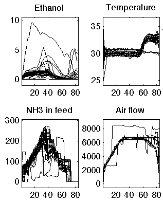
An example of batch trajectory data, in matrix , where there are 4 variables, recorded at 80 times points, on about 20 batches is shown here:
Data fusion
This is a recent buzz-word that simply means we collect and use data from multiple sources. Imagine the batch system above: we already have data in recorded by manual entry, data in recorded by sensors on the process, and then , typically from lab measurements. We might even have a near infrared probe in the reactor that provides a complete spectrum (a vector) at each point in time. The process of combining these data sets together is called data fusion. Each data set is often referred to as a block. We prefer to use the term multiblock data analysis when dealing with combined data sets.
The most outstanding feature of the above data sets is their large size, both in terms of the number of rows and columns. This is primarily because data acquisition and data storage has become cheap.
The number of rows isn’t too big of a deal: we can sub-sample the data, use parallel processors on our computers or distributed computing (a.k.a. cloud computing) to deal with this. The bigger problem is the number of columns in the data arrays. A data set with columns can be visualized using pairs of scatterplots; this is manageable for , but the quadratic number of combinations prevents us from using scatterplot matrices to visualize this data, especially when .
The need here is for a tool that deals with large .
Lack of independence
The lack of independence is a big factor in modern data sets - it is problematic for example with MLR where the becomes singular as the data become more dependent. Sometimes we can make our data more independent by selecting a reduced number of columns, but this requires good knowledge of the system being investigated, is time-consuming, and we risk omitting important variables.
Low signal to noise ratio
Engineering systems are usually kept as stable as possible: the ideal being a flat line. Data from such systems have very little signal and high noise. Even though we might record 50 Mb per second from various sensors, computer systems can, and actually do, “throw away” much of the data. This is not advisable from a multivariate data analysis perspective, but the reasoning behind it is hard to fault: much of the data we collect is not very informative. A lot of it is just from constant operation, noise, slow drift or error.
Finding the interesting signals in these routine data (also known as happenstance data), is a challenge.
Non-causal data
This happenstance data is also non-causal. The opposite case is when one runs a designed experiment; this intentionally adds variability into a process, allowing us to conclude cause-and-effect relationships, if we properly block and randomize.
But happenstance data just allows us to draw inference based on correlation effects. Since correlation is a prerequisite for causality, we can often learn a good deal from the correlation patterns in the data. Then we use our engineering knowledge to validate any correlations, and we can go on to truly verify causality with a randomized designed experiment, if it is an important effect to verify.
Errors in the data
Tools, such as least squares analysis, assume the recorded data has no error. But most engineering systems have error in their measurements, some of it quite large, since much of the data is collected by automated systems under non-ideal conditions.
So we require tools that relax the assumption that measurements have no error.
Missing data
Missing data are very common in engineering applications. Sensors go off-line, are damaged, or it is simply not possible to record all the variables (attributes) on each observation. Classical approaches are to throw away rows or columns with incomplete information, which might be acceptable when we have large quantities of data, but could lead to omitting important information in many cases.
In conclusion, we require methods that:
are able to rapidly extract the relevant information from a large quantity of data
deal with missing data
deal with 3-D and higher dimensional data sets
be able to combine data on the same object, that is stored in different data tables
handle collinearity in the data (low signal to noise ratio)
assume measurement error in all the recorded data.
Latent variable methods are a suitable tool that meet these requirements.